-
Emmanuel
Bacry
Centre de Mathematiques Appliquées
Ecole Polytechnique 91128 Palaiseau Cedex - France
-
Nicolas
Decoster (for
the convolution command only)
Formerly at CRPP Avenue Schweitzer, 33600 Pessac France.
email : decoster@crpp.u-bordeaux.fr
-
Xavier
Surraud (for the convolution command only)
Formerly at Centre de Mathematiques Appliquées
Ecole Polytechnique 91128 Palaiseau Cedex - France
Description
The signal package defines the
signal structure (of type &signal) and includes all the commands
that deal with signals. It also includes the definition of the graphic class
GraphSignal that allows to display signals.It includes some high-level
math functions such as a powerful convolution command (that deals with border
effects and that can use either an fft algorithm fast convolution algorithm
or a direct convolution algorithm.
Examples
Display
of signals
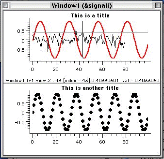
This is the graphic output of the demo command DemoSignalDisp.
This display is basically generated by the code
# Generate
the3 signals
s1 = [sin 100 4]
s2 = .2*Grand(80)
s3 = [sin 100 6]
# Display the signals
disp {{s1 s2}} s3 -..1 -fg 'red' -pen 2 -..3 -curve 'o' -3 -..fv1 -title "This
is a title" -..fv2 -title "This is another title"

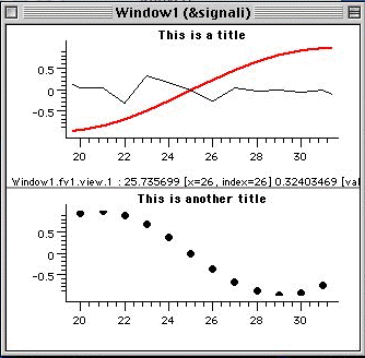
If you perform a zoom using the mouse (or using a disp
command) on a graph, the other graph is automatically synchronized, e.g.,

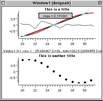
Then, using the mouse you can draw lines or perform linear fits
on one of a signal that is displayed, e.g. on the red signal,

Repeating a signal
To create a signal s1 which is made of the signal s repeated 3 times
you can do
a> s
= <1,2>
= <1,2>
a> s1 = <s,s,s>
= <size=6;1,2,1,2,1,2>
or, using listv's
a> s1 = <{s}*3>
= <size=6;1,2,1,2,1,2>
or, using periodic border effects along with extraction
a> s1=s[*bper,0:5]
= <size=6;1,2,1,2,1,2>
Basic signal extraction
a> s
= <1,3,4,7,10,20>
a> s[1]=<12,13>
** Error : Size of both handsides should match (left size = 1, right size =
2)
---> s[1]=<12,13>
a> s[1,3]=<12,13>
= <size=6;1,12,4,13,10,20>
a> s[1:2,5]={<0,1> <2,2>}
= <size=7;1,0,1,13,10,2,...>
a> print s
s =
0 1
1 0
2 1
3 13
4 10
5 2
6 2
a> s[1:2,3:4]:={<1>}
= <1,1,1,2,2>
a> s[1:]+=I(4)
= <1,1,2,4,5>
a> s[2:3]:={<>}
= <1,1,5>
a> s[0,2]:=<10,20>
= <10,20,1,10,20>
The find operator returns indices that satisfy the condition:
a> find(s==10)
= <0,3>
a> s[find(s==10)]:=40
= <40,20,1,40,20>
Signal extraction using abscissa
and not indices
a> s
= XY(0:#5:1,2*X)
= <x0=0,dx=0.25;0,0.5,1,1.5,2>
a> s[1]
= 0.5
a> s[*x,1]
= 2
a> s[*x,0.7]
= 1
a> s[*xlin,0.7]
= 1.4
another example:
a> s
= XY(<0.5,2,2.5,10>,2*X)
= <size=4;(0.5/1),(2/4),(2.5/5),...>
a> s[*x,1:10]
= <size=3;(2/4),(2.5/5),(10/20)>
a> s[*xlin,1:1:10]
= <size=10,x0=1,dx=1;2,4,6,8,10,12,...>
Building a sine wave - Extaction using real abscissa
Let us first we build a sine wave on ]0,2pi] sampled with 200 points
a> s
= XY(0!:#200:2*pi,sin(X))
= <size=200,x0=0.0314159,dx=0.0314159;0.0314108,0.0627905,0.0941083,0.125333,0.156434,0.187381,...>
Knowing the signal is periodic, extracting the part in the interval [4pi,6pi]
a> s1=s[*x*bper,4*pi:6*pi]
= <size=200,x0=12.5664,dx=0.0314159;1.74846e-07,0.0314108,0.0627905,0.0941083,0.125333,0.156434,...>
Building a piece-wise constant uniformely sampled function
For that purpose we first need to specify the break points
a> s = XY(<0,2,2,3,5>,<0,0,1,-1,2>)
= <size=5;(0/0),(2/0),(2/1),...>
Let us note that s has a discontinuity at x=2. Now we want to uniformely sample
it using a total of 200 points
a> s1=s[*x,:#200:]
= <size=200,x0=0,dx=0.0251256;0,0,0,0,0,0,...>
As you see, to each break point corresponds a step except for the last
point. The last point of the signal is the only one corresponding to a y-value
of 2. Indeed, as we have already explained, each ``step'' starts from a break
point to the next. If you want this last point to be removed you can just type
a> s1=s[*x,:#200:!]
= <size=200,x0=0,dx=0.025;0,0,0,0,0,0,...>
Or if you want a whole step (of size 1) associated to this point, you could
do
a> s1=s[*x*bcon,:#200:!6]
= <size=200,x0=0,dx=0.03;0,0,0,0,0,0,...>
Building a piece-wise linear uniformely sampled function
a> s = XY(<0,2,2,3,5>,<0,0,1,-1,2>)
= <size=5;(0/0),(2/0),(2/1),...>
a> s1=s[*xlin,:\#200:]
= <size=200,x0=0,dx=0.0251256;0,0,0,0,0,0,...>
Building a piece-wise constant uniformely sampled function
from a y-signal
Let s(t) be the periodic function (of period 4) which is piece-wise constant on
each interval [0,1[, [1,2[, [2,3[, [3,4[ and for which s(0) = 1, s(1) = 5, s(2)
= -1, and s(3) = 0. We want to generate a sample of this function (on 200 points)
on the interval [10,22[ !
a> s = <1,5,-1,0>
= <1,5,-1,0>
a> s1 = s[*x*bper,10:\#200:!22]
= <size=200,x0=10,dx=0.06;-1,-1,-1,-1,-1,-1,...>
