Optimization of the Steklov spectrum

Some introductory stuff on the Steklov spectrum are presented here. Below I present the main idea of the computation method for smooth 2D domains and some numerical results concerning various optimization problems of the Steklov eigenvalues.

The idea of using fundamental solutions came from some papers of Alves and Antunes (like this one). The Steklov case is, in a way, nicer since fundamental solutions, which are harmonic functions do not depend on the eigenvalue, like in the case of the Laplace eigenvalues. The main idea is to search for eigenfunctions $u$ which are of the form $$u = \alpha_1 \phi_1+...+\alpha_n \phi_n $$ where $\phi_i$ are harmonic radial functions with singularities outside $\Omega$. Thus $u$ satisfies the PDE analytically in the interior of the set and it only remains to impose the boundary eigenvalue conditions. This we can only do in a finite number of points $(x_i)$ distributed on $\partial \Omega$. The points $(x_i)$ are chosen uniformly on $\partial \Omega$ and the points $(y_i)$, the singularities of $\phi_i$ are chosen each on the normal to the corresponding $(x_i)$. In this way, imposing the boundary conditions at $(x_i)$ we obtain a generalized eigenvalue problem the solutions of which are the Steklov eigenfunctions.

If we place ourselves in the case where the shape $\Omega$ is star shaped we notice that $\Omega$ can be well parametrized by a radial function $\rho : [0,2*\pi) \to \Bbb{R}_+$. This radial function can be in turn approximated by a truncation of its Fourier series to a finite number of terms: $$ \rho(\theta) \approx a_0+ \sum_{i=k}^m a_k \cos (k\theta)+b_k\sin(k\theta)$$ With the aid of the shape derivative formulas provided in (article wentzel) we can find the derivatives with respect to every Fourier coefficient: $$\frac{\partial \sigma_k}{\partial a_i} = \int_0^{2\pi} \left(|\nabla_\tau u_k|^2 -|\partial_n u_k|^2 -\lambda\mathcal{H}|u_k|^2 \right)\rho(\theta) \cos(i\theta) d\theta $$ $$\frac{\partial \sigma_k}{\partial b_i} = \int_0^{2\pi} \left(|\nabla_\tau u_k|^2 -|\partial_n u_k|^2 -\lambda\mathcal{H}|u_k|^2 \right)\rho(\theta) \sin(i\theta) d\theta $$ In this way we obtain an approximation of the Steklov eigenvalues with a function depending on a finite number of parameters. We can optimize this function using gradient descent algorithms.

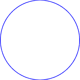
$\displaystyle \min \frac{1}{\sigma_1}+...+\frac{1}{\sigma_n}$ is realized by the disk - perimeter and area constraints;
$\max \sigma_1, \max \sigma_1\sigma_2$ are realized by disks - perimeter and area constraints.
(Conjecture) the maximizers of $\sigma_k$, $k=2,...,10$ with area constraint are connected. The numerical results can be seen below. We observe the following behaviour: optimal eigenvalue are multiple and multiplicity clusters begin at the eigenvalue index. The optimal shapes seem to have dihedral symmetry.
(Conjecture) the product $\sigma_1\sigma_2...\sigma_n$ is maximized by the disk (both constraints). This is known to be true for $n=2$ (Hersch-Payne).
(Conjecture) We say that $A \subset \{0,1,2,3,...\}$ has the property $(P)$ if $1 \in A$ and $2k \in A \Rightarrow 2k-1 \in A$. If $A$ has the property $(P)$ then $\displaystyle \sum_{k \in A}\frac{1}{\sigma_k}$ is minimized by the disk in the case of a volume constraint. For example $\displaystyle \frac{1}{\sigma_1}+\frac{1}{\sigma_3}+\frac{1}{\sigma_4}$ is minimized by the disk in the case of the volume constraint and the perimeter constraint. This was verified for various $A$ with property $(P)$ with $A \subset \{0,1,...,15\}$.
(Conjecture; appears in the article of Hersch-Payne-Schiffer) $\displaystyle \sum_{k=1}^n \frac{1}{\sigma_{2k-1}\sigma_{2k}}$ is minimized by the disk. This was checked numerically in the case of both constraints.

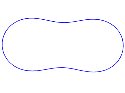
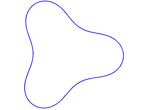
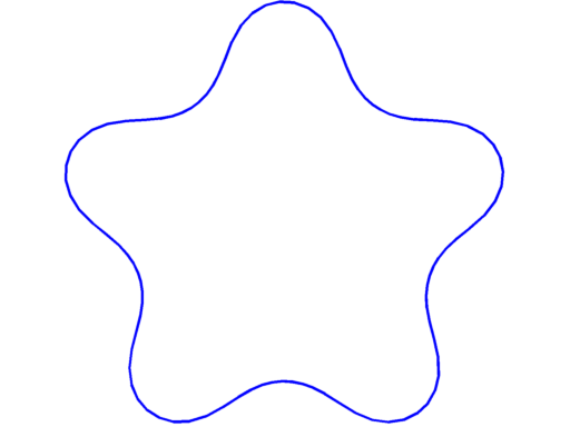
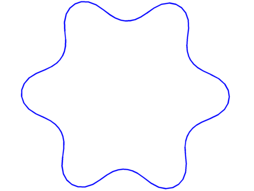
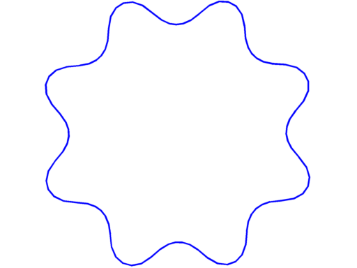
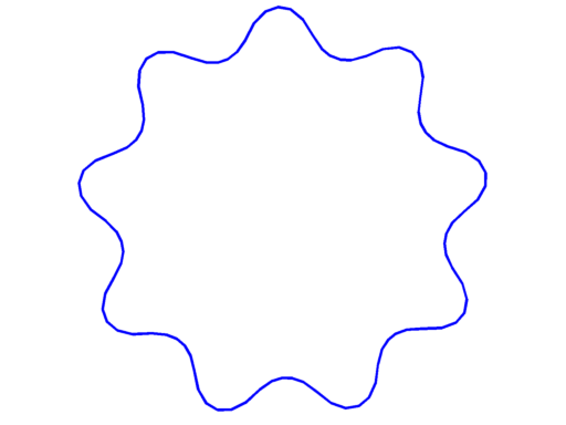
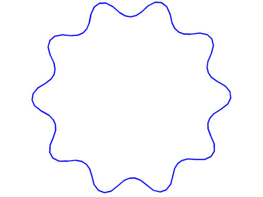
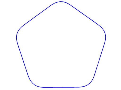
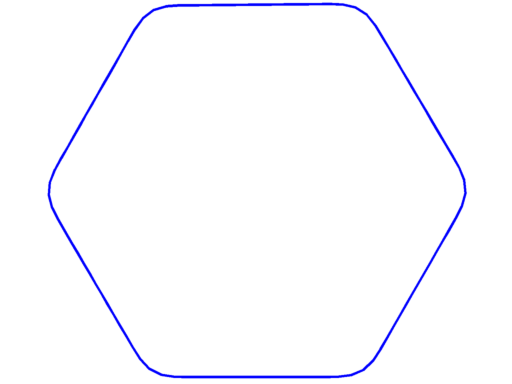
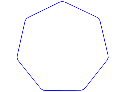
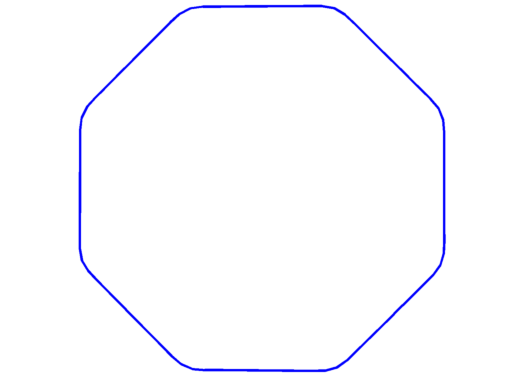
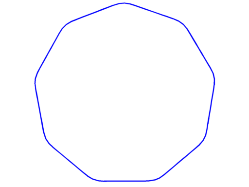
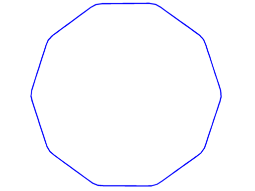
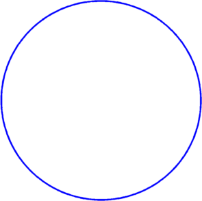
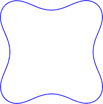
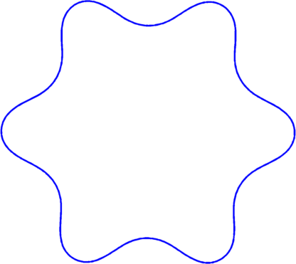
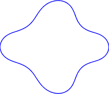
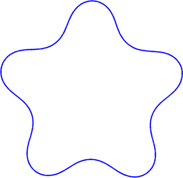
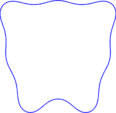
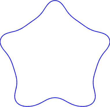
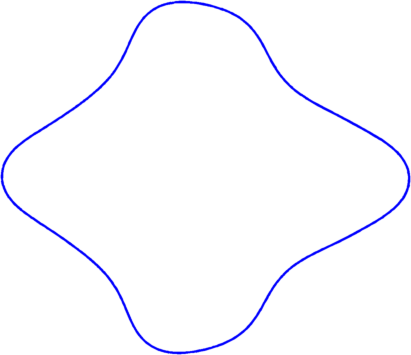
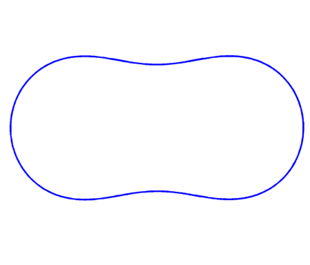
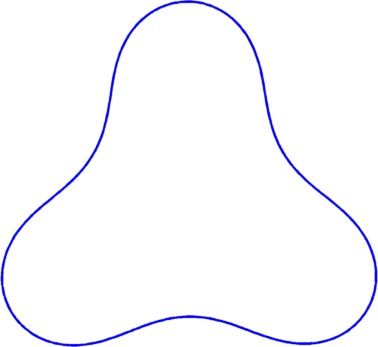
Pictures below are numerical optimal domains which maximize the corresponding Steklov eigenvalue under area constraint.


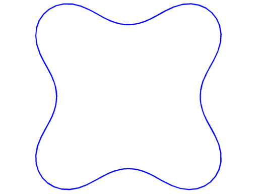$\sigma_2 = 2.91$	$\sigma_3 = 4.14$	$\sigma_4 = 5.28$

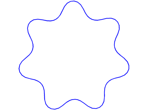$\sigma_5 = 6.49$	$\sigma_6 = 7.64$	$\sigma_7 = 8.84$

$\sigma_8 = 10.00$	$\sigma_9 = 11.19$	$\sigma_{10} = 12.35$

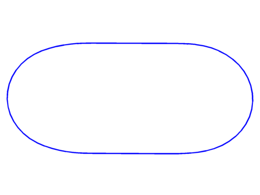
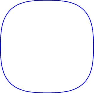
Pictures below are numerical optimal domains which maximize the corresponding Steklov eigenvalue under area and convexity constraint.


$\sigma_2 = 2.87$	$\sigma_3 = 3.86$	$\sigma_4 = 4.56$

$\sigma_5 = 5.61$	$\sigma_6 = 6.24$	$\sigma_7 = 7.43$

$\sigma_8 = 7.99$	$\sigma_9 = 9.15$	$\sigma_{10} = 9.75$

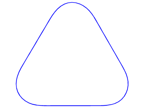
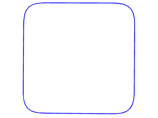
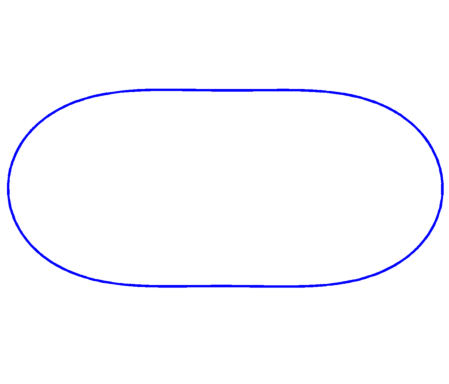
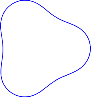
Below are some results concerning the optimization of some general functionals depending on the Steklov spectrum with area constraint.


$\max \sigma_1+\sigma_2 = 3.75$	$\max \sigma_1+\sigma_2+\sigma_3 = 4\sqrt{\pi}$	$\max \sigma_1+...+\sigma_4 = 6\sqrt{\pi}$

$\max \sigma_1+...+\sigma_5 = 9\sqrt{\pi}$	$\max \sigma_1+\sigma_4 = 6.49$	$\max \sigma_1+\sigma_6 = 8.93$

$\max \sigma_4+\sigma_6 = 10.8$	$\max \sigma_5+\sigma_6 = 12.99$	$\max \sigma_4+\sigma_7 = 11.86$

$\min \frac{1}{\sigma_1}+\frac{1}{\sigma_4} = 0.82$	$\min \frac{1}{\sigma_3}+\frac{1}{\sigma_5} = 0.46$	$\min \frac{1}{\sigma_5}+\frac{1}{\sigma_{11}} = 0.26$

$\min \frac{1}{\sigma_4}+\frac{1}{\sigma_6} +\frac{1}{\sigma_{10}}= 0.49$	$\max \sigma_2\cdot \sigma_3 =8.69$	$\max \sigma_3\cdot \sigma_4 =17.18$

Created: Oct 2015