Permanent Impact has a confounder

Information, via consensus

I have students asking questions about the Permanent Market Impact. Here is the context: you are a large asset manager and you have to buy or sell a large amount of share today. This instruction is commonly named a metaorder. Now you (or your dealing desk) is going to different trading facilities to chase liquidity, doing that, you (almost) continuously exert a price pressure: you push the price up (or down). As a consequence the price get worst for you (the more you buy, the higher, or the more you sell, the lower).

Definition of the problem

This price move is what we call the Market Impact. It is important to be understood because

• it is part of the price you pay, and as such should be part of your subsequent post-trade, Trade Cost Analysis (TCA)
• if you are a rational trader, you should solve an optimizations that makes the balance between trading slow to minimize this impact and trading fast to be close to your decision price.

For ages we know that Market Impact has three phases:

Moro, Esteban, Javier Vicente, Luis G. Moyano, Austin Gerig, J. Doyne Farmer, Gabriella Vaglica, Fabrizio Lillo, and Rosario N. Mantegna. “Market impact and trading profile of large trading orders in stock markets” (2009).

1. a transient quick, almost linear, growth: high frequency market makers (or the ones with no inventory of size, that is similar) are quickly giving up to resist;
2. a concave phase that is reaching a peak that is the temporary impact of the order;
3. a decay phases until the price reached a steady-state regime: the Permanent Market Impact.

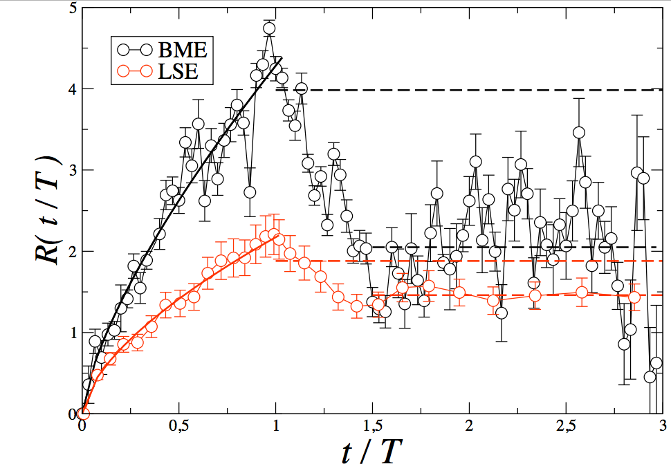
This blog post summarizes the state of the art on this last point.¹ To obtain the upper curve:

• you take all your metaorders longer than 15min and shorter than a day;
• you record the (public) market prices \(p_t\) during their lifetime \([0,T]\) and the usual average bid-ask spread \(\psi\) of the considered stock (trying to not be in sample, a long average of the bid-ask spread over the last 3 months should do the job);
• for each metaorder \(\omega\), you compute the curve \[{\rm sign}(\omega)\frac{p_{uT} - p_0}{\psi},\quad u\in[0,1].\]
• you average them.

A strong conditioning by nature

That is a simple as that. The only difficulty is to get a database of metaorders. Usually traders (asset managers or their dealing desks) have it, but nobody else. Academics have hence difficulties to study the market impact of metaorders, except in association with market participants. This implies a very strong conditioning of the datasets by the instructions (trading bets) of one market participant.

from Briere, Marie, Charles‐Albert Lehalle, Tamara Nefedova, and Amine Raboun. “Modeling transaction costs when trades may be crowded: A Bayesian network using partially observable orders imbalance.” Machine Learning for Asset Management: New Developments and Financial Applications (2020): 387-430.

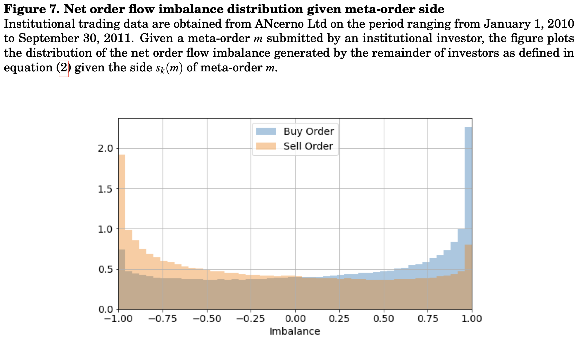
To observe a metaorder, an instruction has to be sent, and hence a portfolio manager has made a bet: that the price will move up² if he buys, or the reverse if he sells. The upper chart shows one of the consequence, using a unique database of around 10% of the metaorders on the US market during decades³: the flow of metaorders is polarised, i.e. on average given I send a buy (resp. sell) metaorder, the other market participants do so. For details, see the paper “Modeling transaction costs when trades may be crowded: A Bayesian network using partially observable orders imbalance” (2020).

What do we observe

The charts like the one of “Market impact and trading profile of large trading orders in stock markets” suggest that: conditionally that I buy (resp. sell), there will be a permanent effect on the price of the traded instrument.

To confirm this sentence is true,

1. one can change the context⁴ to be sure that the shape of the curve is invariant to such modifications. One possible context to change is the cause that triggered the issuance of the metaorder.
2. another active (causal) experiment is to send random orders on the market.

Cash trades do not have permanent market impact

One chart from the Gomes and Waelbroeck paper

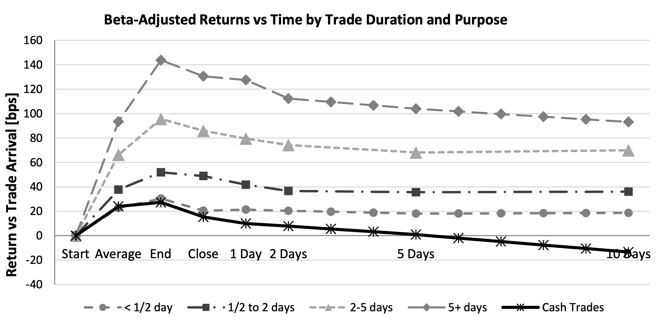
The first approach has been done by Carla Gomes and Henri Waelbroeck. “Is market impact a measure of the information value of trades? Market response to liquidity vs. informed metaorders” Quantitative Finance 15, no. 5 (2015): 773-793. The outcome is clear cash trades do not have market impact. These “cash trades’’ (solid line) stem from the initialisation of a new portfolio, independently from any market-related circumstances.⁵

Random metaorders do not have permanent market impact neither

Despite they do not publish it, several hedge funds experimented random (small) metaorders. What is heard is that these orders have no permanent market impact neither.

Permanent market impact is the expected value of the trade

On most databases of metaorders, more authors found a equilibrium between the average price at which a metaorder obtains its execution and the permanent market impact. Back of the enveloppe, this implies that the permanent price move establishes at 2/3 of the temporary market impact. This is intensively explained with empirical evidences by Bershova, Nataliya, and Dmitry Rakhlin in “The non-linear market impact of large trades: Evidence from buy-side order flow” Quantitative finance 13, no. 11 (2013): 1759-1778.

End of the day market impact, value of the trade and value of the position

If one wants to go further than the value of the trade, and motivated by the fact that if the cost of acquiring of a position corresponds at the level the price establishes there may be no gain to trade, papers looked further than one day ahead:

1. Capital Fund Management’s (CFM, a large systematic French hedge fund) team compared the permanent market impact to the expected value of the position, using that for the combination of predictors that motivated the trades in Brokmann, Xavier, Emmanuel Serie, Julien Kockelkoren, and J-P. Bouchaud. “Slow decay of impact in equity markets” Market Microstructure and Liquidity 1, no. 02 (2015).
2. CA Cheuvreux’ team (the largest French broker at the time, backed by the Investment Bank of Crédit Agricole) did the same: comparing the permanent market impact with the beta of the position, and assuming it is the expected value of the position of its clients’ metaorders.

I will focus more on the second one, simply because I am one of its co-authors.

With Emmanuel Bacry, Adrian Iuga, and Matthieu Lasnier we complemented the usual intraday studies by a daily analysis in “Market impacts and the life cycle of investors orders” Market Microstructure and Liquidity 1, no. 02 (2015).

Main daily chart of “Market impacts and the life cycle of investors orders”

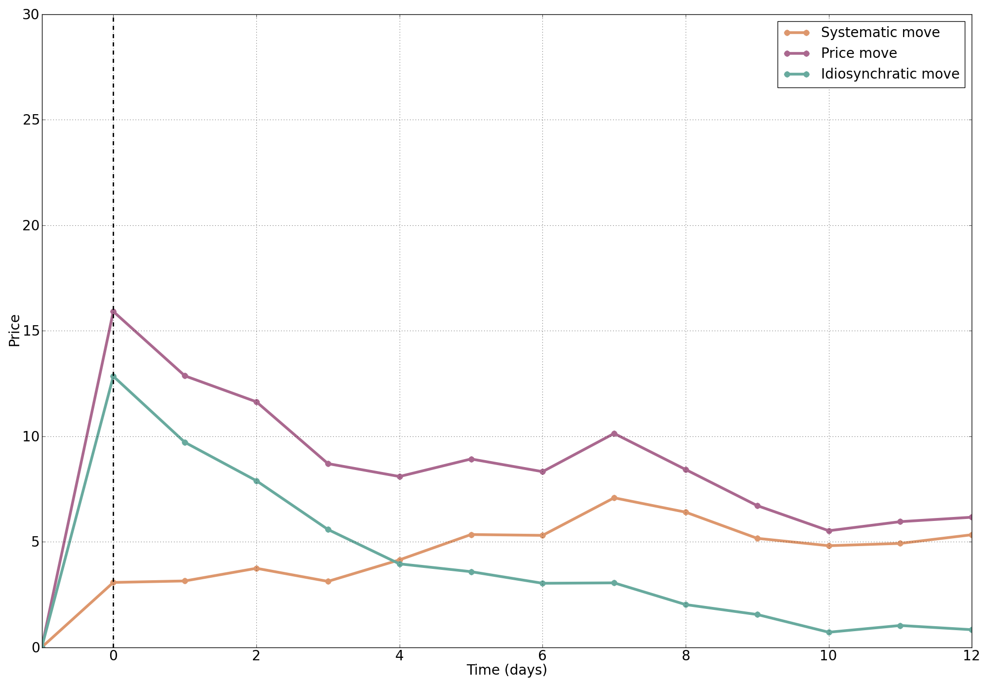
The upper chart is the daily price move relative to the price before the start of the execution of the metaorder, days after it has been traded. The row daily price move (purple) is decomposed in two components

• the price move corresponding to the beta of the position (assumed to be the bet of the investor) in yellow
• and the remaining in green.

Like the CFM paper, ours provide an evidence that if you remove the expected value of the position, the Permanent Impact decreases to zero in around 10 days.

Note that it is not easy to obtain such a clean chart, because one need to account for autocorrelation of the metaorders: conditionally to the fact there is a metaorder today in my database, there will be another one tomorrow with a high probability –this average auto-correlation was around 30% at the time–, hence one needs to “de-convolute” the daily price moves fron this market impact. See the paper for details.

The value of the position continues to adjust after the trade

Hopefully the charts suggest that the permanent market impact (measured intra-day at the end of the metaorder) is only the start of a move that is the reason that triggered the trade: it will continue to move up (if one bought) day after day (this is the yellow curve on the chart) until the prediction will revert and the asset manager will unwind (paying market impact once more, but getting the value of the bet).

The cause of the permanent market impact precedes the execution of the metaorder

Putting side to side all these evidences

1. there is no permanent market impact (or at least it cannot be statistically distinguished from zero) when there is no informative content in the trade
2. once you removed the expected bet, the impact decays to zero.

These points advocate for the following conclusion: the cause of the permanent market impact precedes the execution of the metaorder. The causal chain is the following:

flowchart LR
  A[Expected move] --> B(Metaorder)
  B --> D[temporary Market Impact]
  A --> C[permanent Market impact]
  C --> E(visible price move)
  D --> E

That is not:

flowchart LR
  B(Metaorder) --> D[temporary Market Impact]
  B --> C[permanent Market impact]
  C --> E(visible price move)
  D --> E

To say it differently: even if your execution system is broken or if your dealing desks does not work today, your decision will have a permanent market impact. This is compatible with Sanford Grossman and Joseph Stiglitz famous paper “On the impossibility of informationally efficient markets” (in The American economic review 70, no. 3, 1980): if you did your homework to understand the information that change the underlying value of a tradable instrument, its price will move to give you the occasion to be rewarded for your effort. All these papers suggest this informational effect is the permanent market impact.

A linear view on Permanent Market Impact

It is time to come back to Jim Gatheral’s paper “No-dynamic-arbitrage and market impact” (Quantitative finance 10, no. 7, 2010): if this permanent market impact exists, it has to be linear in the traded quantity. What we suggest here is that this linearity should come from the decision process deducing the quantity to trade from predictions. This is, by the way, what Kyle’s model assumes in “Continuous auctions and insider trading” Econometrica: Journal of the Econometric Society (1985): 1315-1335.

Mixing linear and square root impacts

At the beginning of this post, I announced in a footnote to stay away from the square root law, but I have to add here that this combination of linear permanent impact with square root temporary impact may create empirical confusions, depending on the amount of information contained in the metaorders of your database. Say that if you have metaorders chasing analysts recommendations (that are quickly impacting the price for at least one decade) your market impact model will be dominated by a linear effect, while of you have a database of cash trades, the square root effect will dominate…

A consensus view on Market Impact

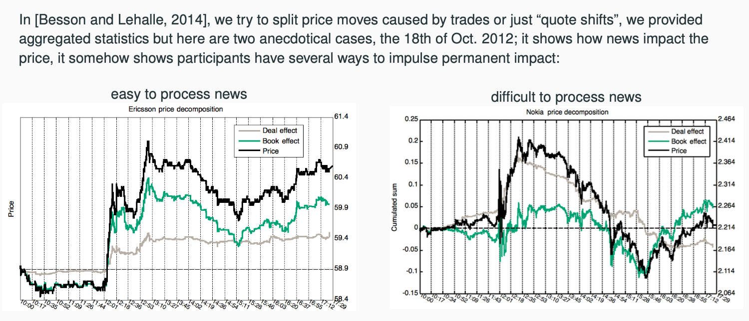
In our white paper with Paul Besson “The deal/book split analysis: A new method to disentangle the contribution to market and limit orders in any price change” (2014) we provided a way to disantangle the effect of liquidity provision and liquidity consumption on price formation. Going away from metaorders for a minute (but with some work it can be linked to them), we provide empirical evidences that

• when there is a consensus between buyers and sellers: the price moves, most often without any transaction, and stay there: this is Permanent and Informational Market Impact (left panel of the picture below)
• whereas when there is not, thus when price moves are mostly driven by aggressive liquidity consumption, then the effect is temporare (right panel).

A slide from my course at the Probabilités et Finance Master Program of Polytechnique and Paris 6 (2024)

This has to be added to the story of metaorders since we now have to talk about informational vs. mechanical move, that can be stylized as the traditional view of economists (price discovery) vs. econophysicists (price formation).

Implications

For TCA (Transaction Cost Analysis)

When a broker or an asset manager (or its dealing desk) is involved in pre-trade or post-trade analysis, or TCA, it is now clear that the model they use to anticipate or explain the cost of a portfolio of trades should incorporate an indicator of the expected informational content of the trade.

Similarly to market makers performing ’‘toxicity analysis’’ of their client flows, any market impact model for TCA should be augmented by a level of informativeness of the trade. Otherwise, market impact models are doomed to be only applicable to the average client mix of the broker, meaning that it contains the average level of information of her clients, and hence reflects the level of informativeness of none of them…

For optimal execution

The standard frameworks for optimal execution are made to help to compute the adequate balance between trading slow enough to not suffer from market impact and trading fast enough to get a price close to the decision price.

The usual way it is implemented on trading speed⁶

• the trading speed \(\nu\) is time continuous, thus the inventory \(Q\) varies following \(dQ=\nu\,dt\)
• for a price \(S\), the cash account of the trader evolves accordingly to \(dX = \nu S\,dt - L(\nu)\,dt\) where \(L(\nu)\) is a frictional costs,mostly referred to as temporary impact
• the price moves accordingly to \(dS = -b(\nu)\,dt + \sigma\,dW\), where \(b(\nu)\) is meant to quantify the permanent market impact;
• on the top of it a risk aversion term is introduced in the cost function, that usually looks like (\(A\) is a penalizing function, often quadratic) \[V(t,x,s,q)=\sup_\nu \mathbb{E}\left[X^\nu_T + A(Q^\nu_T) - \phi\int_{s=t}^T (Q^\nu_s)^2\,ds \middle| X_t=x, S_t=s, Q_t=q\right].\]

It says that you start with a long position \(Q_0>0\) that you sell at the speed of \(\nu\) shares per second, that your cash account increases (but with a penality that corresponds to the temporary market impact) and the price goes down following a permanent market impact term. It adds a valorisation of the remaining position \(Q_T\) at terminal time and a running cost term (in factor of the risk aversion coefficient \(\phi\)) that pushes the trader to finish quickly.

What we are saying there is that the permanent market impact term \(b(\nu)\) should not be a function of the instantaneous trading speed, since it is not caused by it but it is caused by the same factor that created the sell metaorder of since \(Q_0\). If we believe that the size of this metaorder is linear in the expected price move \(\widehat{\Delta} P\) that triggered the decision, we should probably replace \(b(\nu)\) by something like \[b(\nu)\leadsto b\, \frac{\widehat{\Delta} P}{T},\] to express that, whatever we do: it is too late to do anything that will change the permanent market impact, since it is linked to the decision and its fate has been sealed earlier in the process.

Open questions

This post is not to say that everything is done and understood. That are remaining mysteries; for instance

1. Can we really empirically link the available information and permanent market impact (i.e. subsequent price move)? it relates to find empirical evidences of Sanford Grossman and Joseph Stiglitz 1980 paper, keeping in mind that maybe “Black was right: Price is within a factor 2 of value” (see Bouchaud, Jean-Philippe, Stefano Ciliberti, Yves Lempérière, Adam Majewski, Philip Seager, and K. Sin Ronia (2017)).
2. It suggests studies working on separating the informational (exogenous) price moves from the mechanical (endogenous) ones. They are two interesting papers on the topic
   • Marcaccioli, Riccardo, Jean-Philippe Bouchaud, and Michael Benzaquen. “Exogenous and endogenous price jumps belong to different dynamical classes” Journal of Statistical Mechanics: Theory and Experiment 2022, no. 2 (2022): 023403.
   • Aït-Sahalia, Yacine, Chen Xu Li, and Chenxu Li. So many jumps, so few news. No. w32746. National Bureau of Economic Research, 2024.
3. Multi-channelled market impact: what is the story when you have a decision flow more fragmented than on cash equities? How to revisit the journey of information and flows (and their effect on prices) when you have old-style market markers, RFQ, inter-dealer markets, etc?

Last but not least, there is a small probability that even if seen from the perspective of each metaorder, and once corrected from the information, the permanent market impact decays to zero statistically (meaning that there is not statistically significant deviation from zero), its re-aggregation over all the metaorders of the day does not.

Footnotes

1. Be careful, this concave curve is not the square root law of the temporary impact: it is simple its averaged evolution in time.

2. or relatively move up, if the PM implements a relative bet, the PnL of this bet will be in the market impact curve.

3. the ANcerno database, produced by Abel Noser.

4. a relation that is robust with respect to a change of context in invariant, that is statistically more powerful than causal.

5. An example is when a discretionary PM (Portfolio Manager) having a portfolio \(\pi(0)\) leaves an asset manager, the newly hired PM may not want to start with the same portfolio, she or he designs a new portfolio \(\pi(1)\) and the asset manager delegates a company to implement the transition, that is buying \(\pi(1)-\pi(0)\): these are the cash trades.

6. see our Mean Field Game paper on the topic and references therein: Cardaliaguet, Pierre, and Charles-Albert Lehalle. “Mean field game of controls and an application to trade crowding” Mathematics and Financial Economics 12 (2018): 335-363) has (here for a sell metaorder).