Detection of Exogenous Price Moves: Localising the Queue Reactive Model
Liquidity dynamics
Charles-Albert Lehalle 
Detecting Exogenous Price Dynamics Thanks to the Queue Reactive Model
Students of the 3rd year of Ecole Polytechnique have the opportunity to get a 3 or 6 months project all “initiation to research” (the codename is EA). I mentored 3 groups in 2024-2025, one of them only spanned 3 months, but the students were (as expected) excellent and they could perform an early exploration of the capability of the Queue Reactive model to detect exogenous price dynamics.
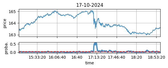
Figure 1: The price (up) and the QRM anomaly contrast (bottom), for the annouce of a new CTO (see lower for details).
The Queue Reactive Model 101
The Queue Reactive Model (QRM) is a model for orderbook dynamics we published in 2015 with Mathieu Rosenbaum and Weibing Huang (during his PhD thesis) Simulating and analyzing order book data: The queue-reactive model. The rational of the QRM is rooted in a 2011 paper about uncertain bands A new approach for the dynamics of ultra-high-frequency data: The model with uncertainty zones (and its capability to predict price jumps and oscillations due to the tick size), and a 2013 paper by Rama Cont and Hadrien de Larrard on the way prices moves can be related to decrease of quantities at first limits (called “order flow” in the paper) Price dynamics in a Markovian limit order market.
Going a few steps further, we imagined that price moves could be explained by three types of events {A, C, T} (Addition or Cancellation of quantity and Transactions), and that the probability of occurence of each event should be a function of the shape of the orderbook.
In the paper, we explored different ways to encode (one would say “embed” today) the shape of the orderbook, and we discovered that it was largely enough to capture and simulate with accuracy liquidity dynamics, the associated mid price volatility was far too low than required. Surprisingly (at the time) the orderflow paper has the reverse feature: good at reproducing volatility but bad at getting the full liquidity dynamics (we are talking about the distribution of the shapes of the orderbook).
The answer to this apparent paradox is that orderbook dynamics are producing deeply mean reverting price dynamics (it is linked to the fact that “conditionally that the first limit depletes, the second limit that is promoted as a first limit is very large, and pushes the price in a reverting direction). One way to solve this is to add a parameter in the model: when the best bid or ask queue is fully consumed, toss a coin and use it to decide if market participants accept to continue the current liquidity dynamics, or if they “reset their views”. In the later case they accept the price change. On the French stocks we looked at the time, this “probability of reset” was around 12%.
A new understanding of the QRM “reset probability”
Since the QR paper, Mathieu and myself continued explorations and published several papers connected to market impact and price formation. I have personally been impressed by the accuracy of an old prediction of Jim Gatheral in his Non-dynamic Arbitrage paper: permanent market impact should be linear No-dynamic-arbitrage and market impact. Understood in conjunction with my 2014 work with Paul Besson on making the difference between price moves due to liquidity consumption (‘deals’) and liquidity displacement (‘book moves’) The deal/book split analysis: A new method to disentangle the contribution to market and limit orders in any price change and with a 2020 paper on the causes of market impact with Amine Raboun, Marie Brière and Tamara Nefedova Modeling transaction costs when trades may be crowded: A bayesian network using partially observable orders imbalance, it became highly probable to me that
- Permanent market impact comes from an agreement of all market participant about exogenous information (like important and easy to understand News),
- While temporary market impact (that mean reverts) comes from a disagreement of market participants.
The reset probability of the QR model could thus model this agreement between market participants: they agree to set the price around anew value because they all have the same understanding of a New, or any similar exogenous information.
The non randomness nature of the QR reset
If it is true, then the realisations of this “reset probability” should not be uniformly distributed. What I mean in that the 12% of reset during a trading day of 6:30 hours not occurred around every 47 minutes (that is 12% of 6h30), they should be clustered around the arrival of “exogenous information”.
This is what I proposed to the two students, Edouard LAFERTE and Janis AIAD: to test if we could “localise” the realisations of the QRM “reset”.
Localisation of Resets
This project was far from easy, first they had to inderstand the format of the Databento level II tick by tick data, especially the provider_id, and then the challenge was to fit a Queue Reactive model on the data.
The spirit of the QRM
As I wrote earlier, the QRM model claim is that the intensity of the processus of occurence of the tree main events {A,C,T} is a function of the orderbook shape. There is thus freedom on how to embed the shape in a feature space that has a lower dimension that the full shape of the book (if you consider 4 limits, you immediately get 8 dimensions, and you have to make a choice for the discretisation of the queue sizes).
Following Occam’s razor in making the model as simple as possible, the shape of the ordebook is encoded by its imbalance. The role of the imbalance in influencing the new move of market participants is well know; it is for instance described in the empirical section of Incorporating signals into optimal trading.
What does it means in practice
- the occurrence of the next trade, cancel or add on the first bid or the first ask if a function of the imbalance of the queues, i.e. of \(I=(Q_A-Q_B)/(Q_A+Q_B)\)
- as a consequence, you ‘simply’ need to get a good estimate of \(\lambda^C(I)\), \(\lambda^A(I)\), and \(\lambda^T(I)\), that are the intensities of three Poisson process driving the observation of Cancellation, or Addition, or Transaction on this queue.
Once it is done: you observe the imbalance of the orderbook at any time, and predict that the next event will occur following these three processes, that are perfectly well-defined once you know the imbalance.
A contrast to identify the need for a reset
We made the following assumption: “a reset should occur when a Queue Reactive Model estimated with a probability of reset set to zero is no more likely to be correct”. In other word, we god the following process to detect empirically the reset time
- Edouard and Janis calibrated a Queue reactive model with a probability of reset set to zero (it means this model is mean reverting too much);
- Each time an event (Cancel, Add, or Trade) occurs, they go back in time and look at the imbalance;
- They computed the likelihood of this occurence.
Setting a threshold to the contrast
This contrast is quite interesting since it is a likelihood: we know that this contrast reaches a level \(\alpha\) with a probability \(q_\alpha\) that is given by the distribution of the corresponding Poisson process of our fitted Queue Reactive.
Since the observations of these stopping time correspond to censored statistics (i.e. you only observe the first of these 3 times on both sides of the book), one way to obtain \(\alpha\) when you choose for instance \(q_\alpha=5\)% is to perform Monte-Carlo simulations. Because of the short time they had, Edouard and Janis decided to use the empirical database in place of Monte-Carlo simulations.
Testing the localisation of the occurrences of the reset
Dear reader, you close to the end of the process
- you know how to fit a queue reactive model on the imbalance (with a reset probability of zero);
- you understand how to compute the likelihood of this model, that will be our contrast \(C(t_i)\) for any stopping time \(t_i\) at which an event occured;
- you know an empirical way to get the threshold \(\alpha_{0.05}\) to apply so that the likelihood will reach this threshold 5% of the time.
The last step is to use a sliding windows (of \(K=120\) events for instance) and to measure how many times \(\alpha(0.05)\) is crossed among these 120 events. The formula is \[f_i(\alpha) = \frac{1}{K}\sum_{k=1}^K \delta[C(t_{i-k-1})<\alpha_{0.05}].\]
This fraction of event should be, in theory, equal to 5%. It is of course true on average, the question we ask now is: is \(f_i(\alpha)\gg 5\)% by clusters or uniformly in time?
If they are some time interval \((t_i,t_j]\) during which \(f_i(\alpha)\gg 0.05\) (call them Active intervals), and others where \(f_i(\alpha)\simeq 0.05\) call them Endogenous intervals), it means that
- the Endogenous intervals are fully compatible with the Queue Reactive model without reset; a consequence is that the price mean reverts on them;
- the Active intervals are not: something is missing, the Queue Reactive model is not enough: resets are needed.
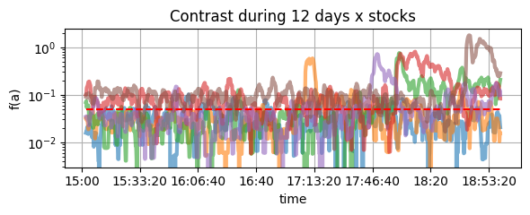
Figure 2: The QRM anomaly contrast (y-log scale) for different days and stocks.
The upper chart is (on a logarithmic scale) the empirical value of \(f_i(\alpha)\): we seem to be in the situation we had in mind initially: When it is greater than 5%, it lasts long (watch the red, green, purple, and orange curves).
Correspondance between clusters of occurence of resets and exogenous information
Now that we suspect the resets happen in clusters, the last step of the reasoning is to try to understand if something specific occurred on the stock that is exogenous. We are not at the stage of a full paper, with a very rigorous control fo all the possible parameters; our goal is to see if the need of a reset for a simple Queue Reactive correspond to the arrival of exogenous information.
That for, Edouard and Janis
- added a chart of the prices
- looked on the web if, during the Active intervals, something easy to understand happened to the underlying company.
To my surprise, the result was a hit rate close to 100%: all the Active intervals correspond to exogenous information, and the days with no Active interval had no inflows of exogenous information. And keep in mind that it is done without looking at the price: only at the rate of occurence of events on the orderbook!
This chart is a typical example:
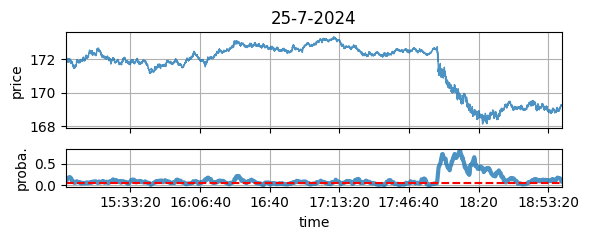
Figure 3: The price (up) and the QRM anomaly contrast (bottom), see later for the details.
A table with examples
| Date | Stock | Price Moves | High Contrast | Exogenous cause |
|---|---|---|---|---|
| 2024-07-25 | Yes | Yes | Yes: Google quarterly results + announcement of chatGPT (Fig. 3) | |
| 2024-08-05 | Yes | Yes | Yes: lawsuit lost by Google for monopolistic practices | |
| 2024-08-29 | Yes | Yes | Yes: Publications of Google’s earnings for Q3 | |
| 2024-09-18 | No | Yes | Yes: (but not idiosyncratic) FED cuts rates (Fig. 4) | |
| 2024-09-20 | No | Yes | Yes: Google has been found guilty of monopolizing the search market by the US Department of Justice | |
| 2024-10-17 | Yes | Yes | Yes: Announcement of a new CTO (Fig. 1) | |
| 2024-11-10 | Yes | No | No |
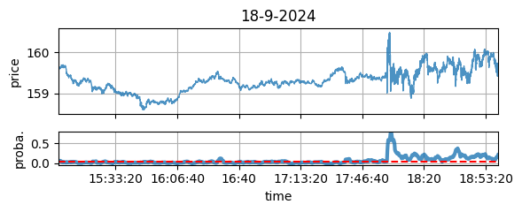
Figure 4: Not idiosyncratic chock (FED’s rates cut), but detected by the QRM contrast.
Next steps
What is exogenous?
To go further, one of the difficulties is to define properly what is an exogenous information. One thing is for sure: we can have a clear understanding of what is endogenous for a QR model with its reset probability set to zero: it means that in the ‘endogenous’ regime all events on the orderbook are triggered by the shape of the orderbook and nothing else.
Non anticipated News (that is something difficult to define, by the way), are exogenous in this sense. But keep in mind that a move of another tradable instrument that is part of the same index can be perceived as exogenous too.
This is just explorations…
Of course, this project is just opening a door, it is now needed to conduct a more systematic exploration, building more rigorous tests than the empirical contrast we used, and use a database of News as a proxy of exogenous information, over years and over a large number fo stocks.