Package installation

The package can be installed from CRAN by

install.packages("ggwordcloud")

or the development version from the github repository

devtools::install_github("lepennec/ggwordcloud")

Please check the latest development version before submitting an issue.

The love / thank you words dataset

Along this vignette, we will use a lovely dataset: a collection of the word love in several language combined with the number of native speakers of those language as well as the total number of speakers. The data have been extracted from wikipedia and is exposed in two data frame of 4 columns: - lang: the ISO 649 language code - words: the word love in those languages - native_speakers: the number of native speakers (in millions) of those languages - speaker: the corresponding total number of speakers (in millions) Another dataset with thank you in several languages is also available. The first one love_words (thankyou_words) contains 147 (133) different languages while the second love_words_small (thankyou_words_small) contains the 34 (34) languages having more than 50 millions speakers.

library(ggwordcloud)
#> Le chargement a nécessité le package : ggplot2

data("love_words_small")
data("love_words")

Word cloud

The geom_text_wordcloud geom constructs a word cloud from a list of words given by the label aesthetic:

set.seed(42)
ggplot(love_words_small, aes(label = word)) +
  geom_text_wordcloud() +
  theme_minimal()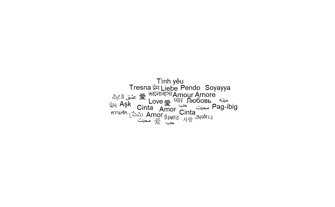

Note that we have used theme_minimal() to display the words and nothing else. The word cloud is, by default, centered and the words are placed along a spiral in a way they do not overlap.

Because there is some randomness in the placement algorithm, the same command can yield a different result when using a different random seed:

set.seed(43)
ggplot(love_words_small, aes(label = word)) +
  geom_text_wordcloud() +
  theme_minimal()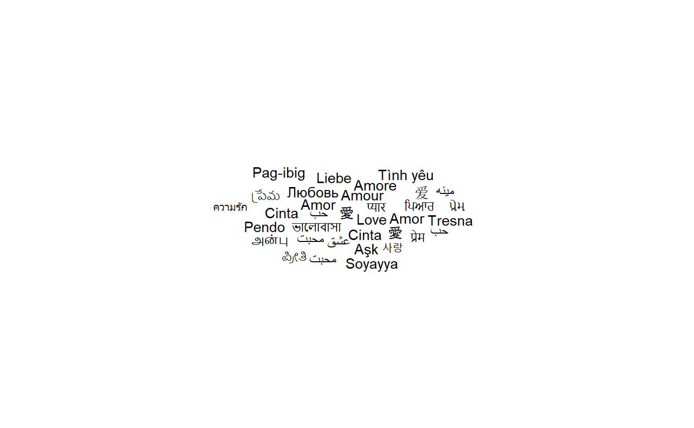

Word cloud and text size

So far all the words had the same size because we do not specify a size aesthetic. If we use the total number of speakers, we obtain:

set.seed(42)
ggplot(love_words_small, aes(label = word, size = speakers)) +
  geom_text_wordcloud() +
  theme_minimal()

The words are scaled according to the value of the size aesthetic, the number of speakers here. There are several classical choices for the scaling: the font size could be chosen proportional to the value or to the square root of the value so that the area of a given character is respectively proportional to the square of the value or the value itself. By default, ggplot2 uses the square root scaling but does not map a value of \(0\) to \(0\).

In order to obtain a true proportionality (and a better font size control), one can use the scale_size_area() scale:

set.seed(42)
ggplot(love_words_small, aes(label = word, size = speakers)) +
  geom_text_wordcloud() +
  scale_size_area(max_size = 30) +
  theme_minimal()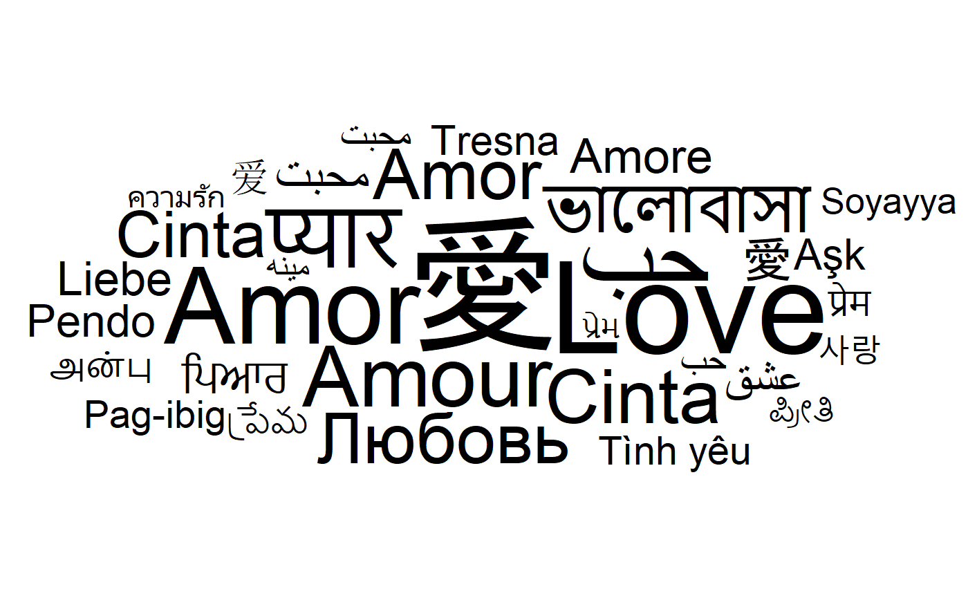

It turns out that both wordcloud and wordcloud2 default to a linear scaling between the value and the font size. This can be obtained with the scale_radius() scale:

set.seed(42)
ggplot(love_words_small, aes(label = word, size = speakers)) +
  geom_text_wordcloud() +
  scale_radius(range = c(0, 30), limits = c(0, NA)) +
  theme_minimal()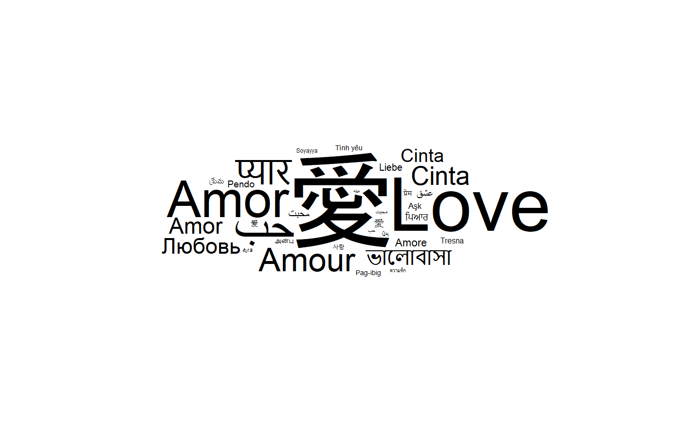

Word cloud and text area

As explained before, by default, this is the size of the font which is proportional to the square root of the value of the size aesthetic. This is a natural choice for a shape as the area of the shape will be proportional to the raw size aesthetic but not necessarily for texts with different lengths. In ggwordcloud2, there is an option, area_corr to scale the font of each label so that the text area is a function of the raw size aesthetic when used in combination with scale_size_area:

set.seed(42)
ggplot(love_words_small, aes(label = word, size = speakers)) +
  geom_text_wordcloud(area_corr = TRUE) +
  scale_size_area(max_size = 50) +
  theme_minimal()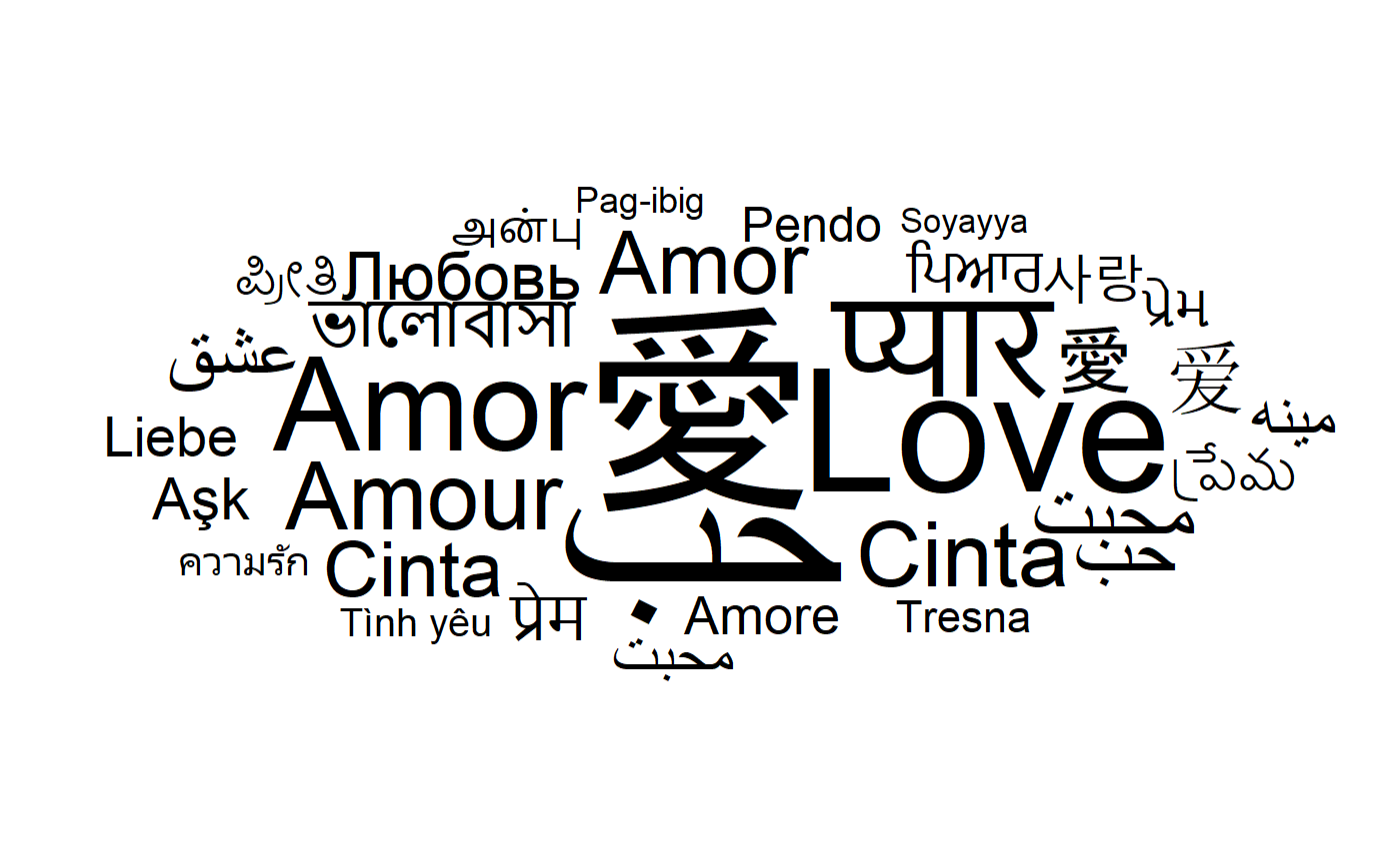

One can equivalently use the geom_text_wordcloud_area geom:

set.seed(42)
ggplot(love_words_small, aes(label = word, size = speakers)) +
  geom_text_wordcloud_area() +
  scale_size_area(max_size = 50) +
  theme_minimal()

By default, the area is proportional to the raw size aesthetic. To better match the human area perception, one can use the power_trans scale with a factor of \(1/.7\):

set.seed(42)
ggplot(love_words_small, aes(label = word, size = speakers)) +
  geom_text_wordcloud_area() +
  scale_size_area(max_size = 50, trans = power_trans(1/.7)) +
  theme_minimal()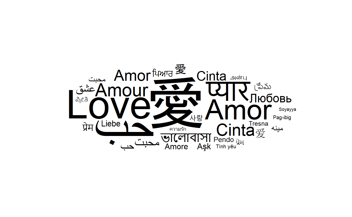

Word cloud with too many words

The non overlapping algorithm may fail to place some words due to a lack of space. By default, those words are displayed at the center of the word cloud and comes with a warning.

set.seed(42)
ggplot(love_words_small, aes(label = word, size = speakers)) +
  geom_text_wordcloud_area() +
  scale_size_area(max_size = 80) +
  theme_minimal()
#> Warning in wordcloud_boxes(data_points = points_valid_first, boxes = boxes, :
#> Some words could not fit on page. They have been placed at their original
#> positions.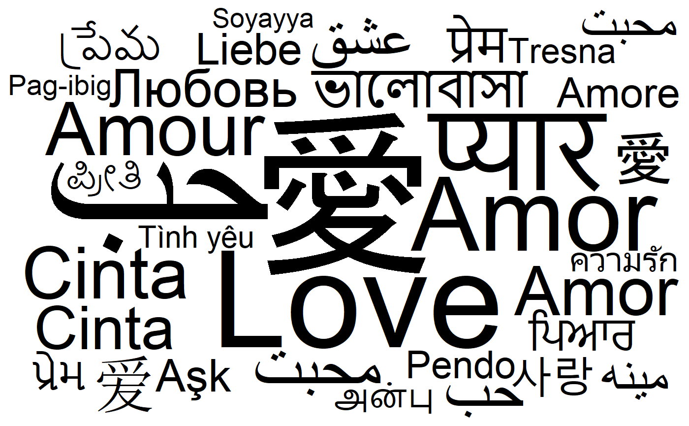

It is up to the user to avoid this issue by either removing some words or changing the size scale. One can also chose to remove those words using the rm_outside option:

set.seed(42)
ggplot(love_words_small, aes(label = word, size = speakers)) +
  geom_text_wordcloud_area(rm_outside = TRUE) +
  scale_size_area(max_size = 80) +
  theme_minimal()
#> Warning in wordcloud_boxes(data_points = points_valid_first, boxes = boxes, :
#> Some words could not fit on page. They have been removed.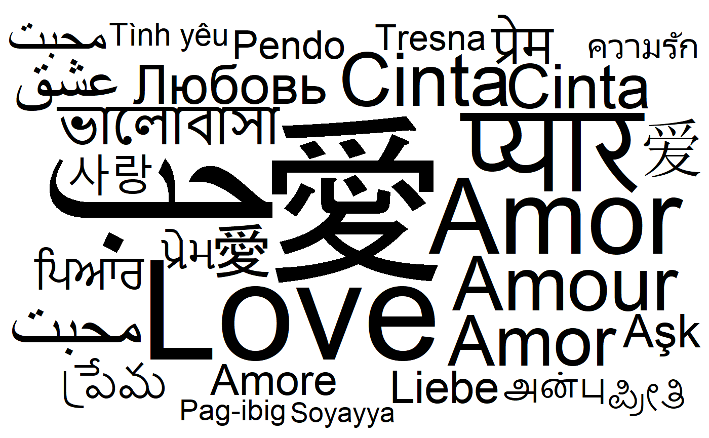

Word cloud and rotation

The words can be rotated by setting the angle aesthetic. For instance, one can use a rotation of 90 degrees for a random subset of 40 % of the words:

library(dplyr, quietly = TRUE)
#> 
#> Attachement du package : 'dplyr'
#> Les objets suivants sont masqués depuis 'package:stats':
#> 
#>     filter, lag
#> Les objets suivants sont masqués depuis 'package:base':
#> 
#>     intersect, setdiff, setequal, union

love_words_small <- love_words_small %>%
  mutate(angle = 90 * sample(c(0, 1), n(), replace = TRUE, prob = c(60, 40)))

set.seed(42)
ggplot(love_words_small, aes(
  label = word, size = speakers,
  angle = angle
)) +
  geom_text_wordcloud_area() +
  scale_size_area(max_size = 40) +
  theme_minimal()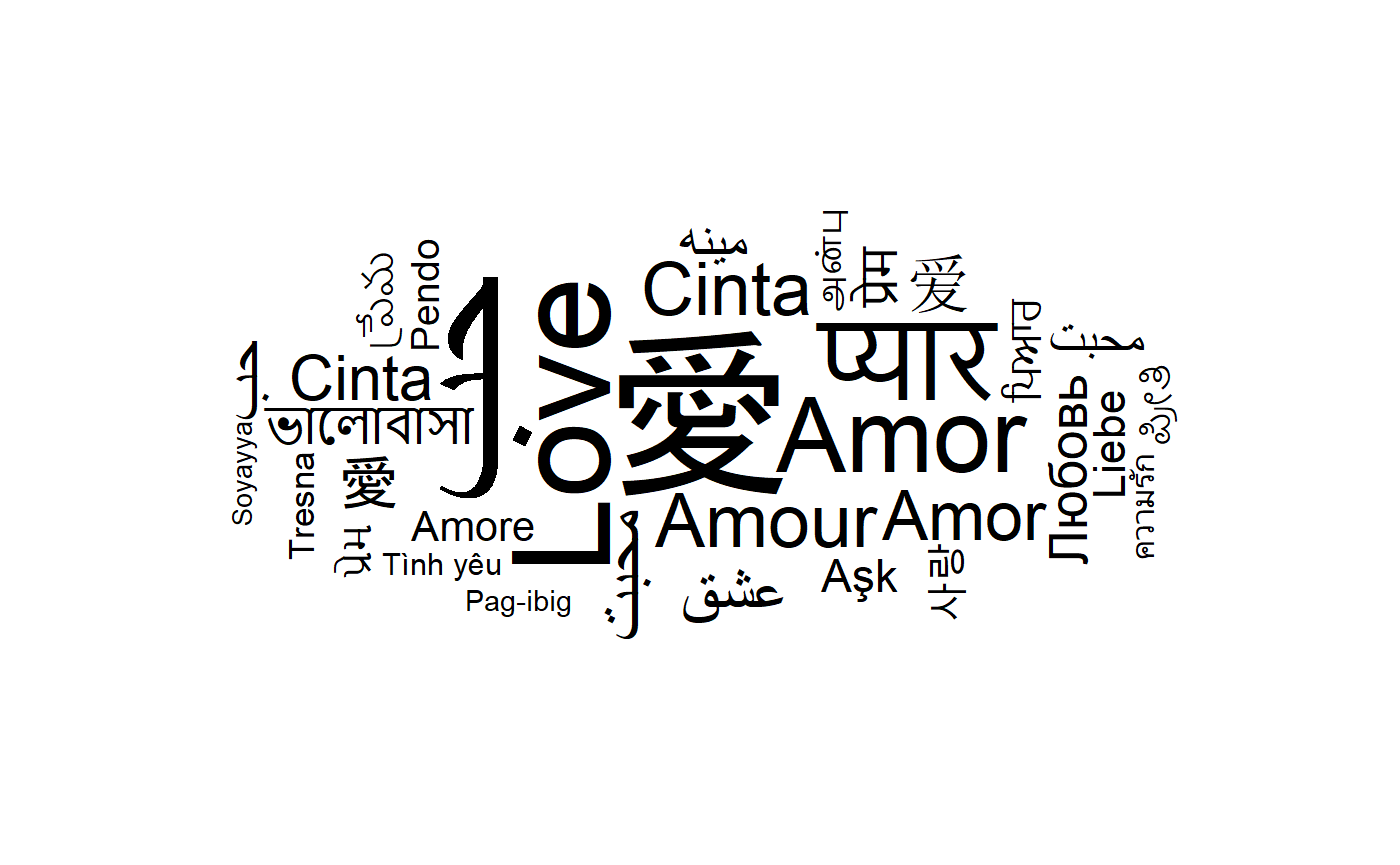

ggwordcloud is not restricted to rotation of 90 degrees:

love_words_small <- love_words_small %>%
  mutate(angle = 45 * sample(-2:2, n(), replace = TRUE, prob = c(1, 1, 4, 1, 1)))

set.seed(42)
ggplot(love_words_small, aes(
  label = word, size = speakers,
  angle = angle
)) +
  geom_text_wordcloud_area() +
  scale_size_area(max_size = 40) +
  theme_minimal()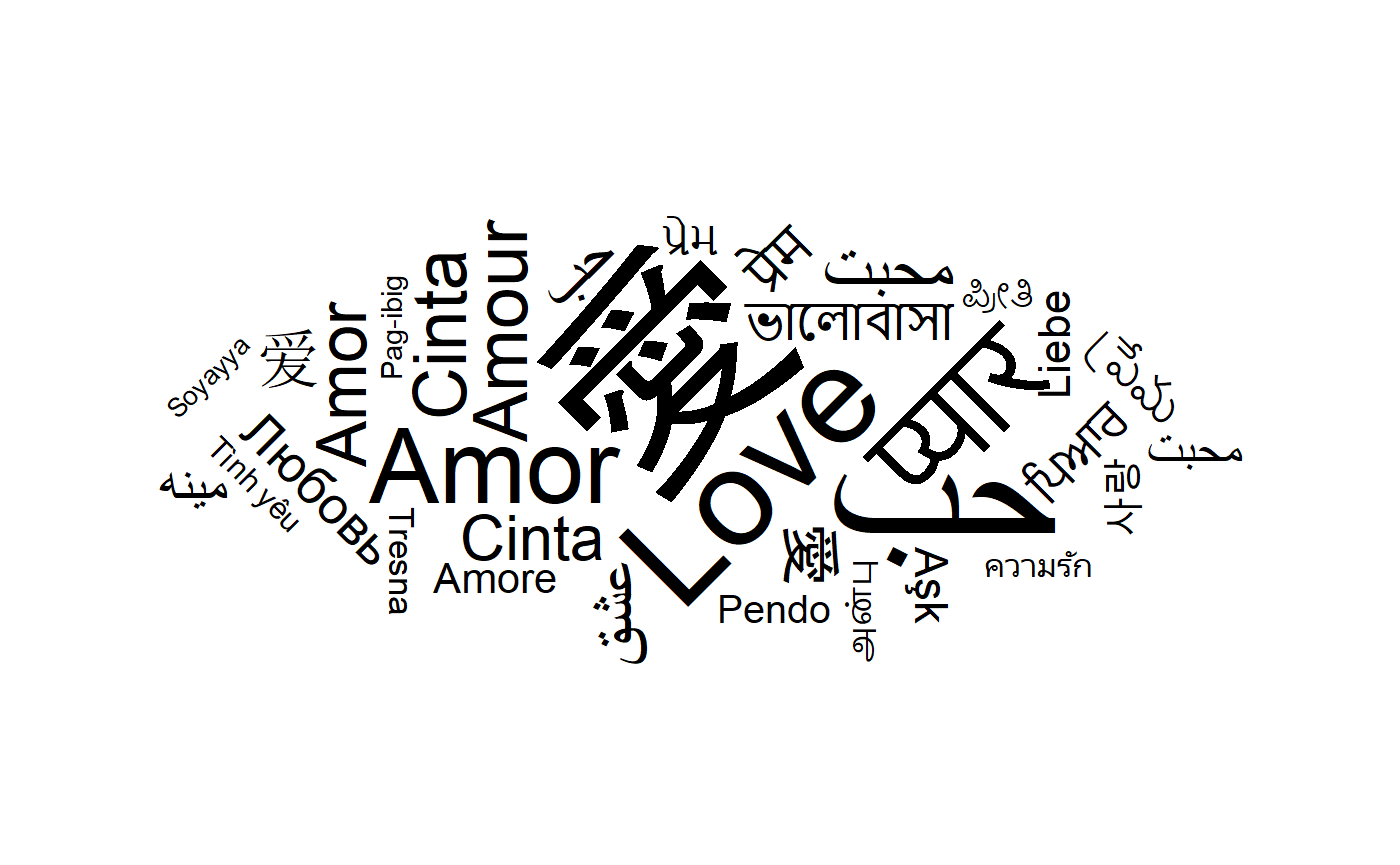

Word cloud and eccentricity

The ggwordcloud algorithm moves the text around a spiral until it finds a free space for it. This spiral has by default a vertical eccentricity of .65, so that the spiral is 1/.65 wider than taller.

set.seed(42)
ggplot(love_words_small, aes(label = word, size = speakers)) +
  geom_text_wordcloud_area() +
  scale_size_area(max_size = 40) +
  theme_minimal()

This can be changed using the eccentricity parameter:

set.seed(42)
ggplot(love_words_small, aes(label = word, size = speakers)) +
  geom_text_wordcloud_area(eccentricity = 1) +
  scale_size_area(max_size = 40) +
  theme_minimal()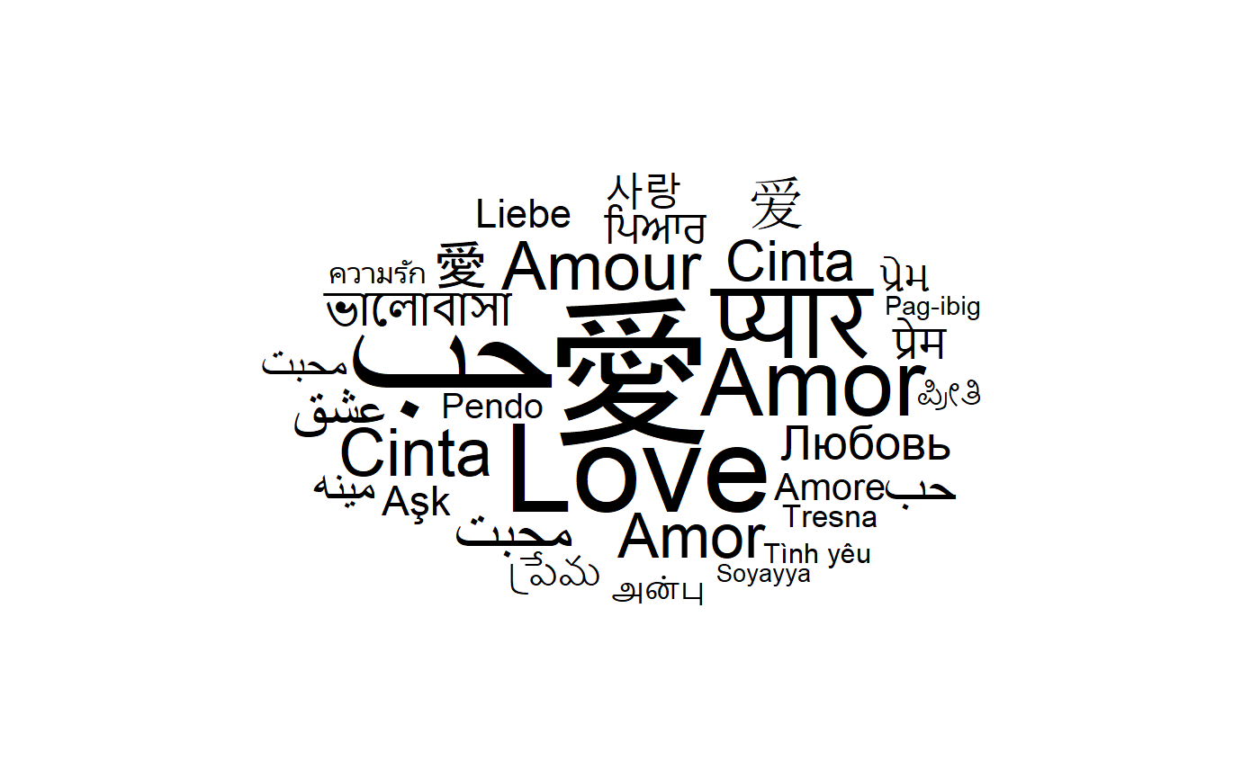

set.seed(42)
ggplot(love_words_small, aes(label = word, size = speakers)) +
  geom_text_wordcloud_area(eccentricity = .35) +
  scale_size_area(max_size = 40) +
  theme_minimal()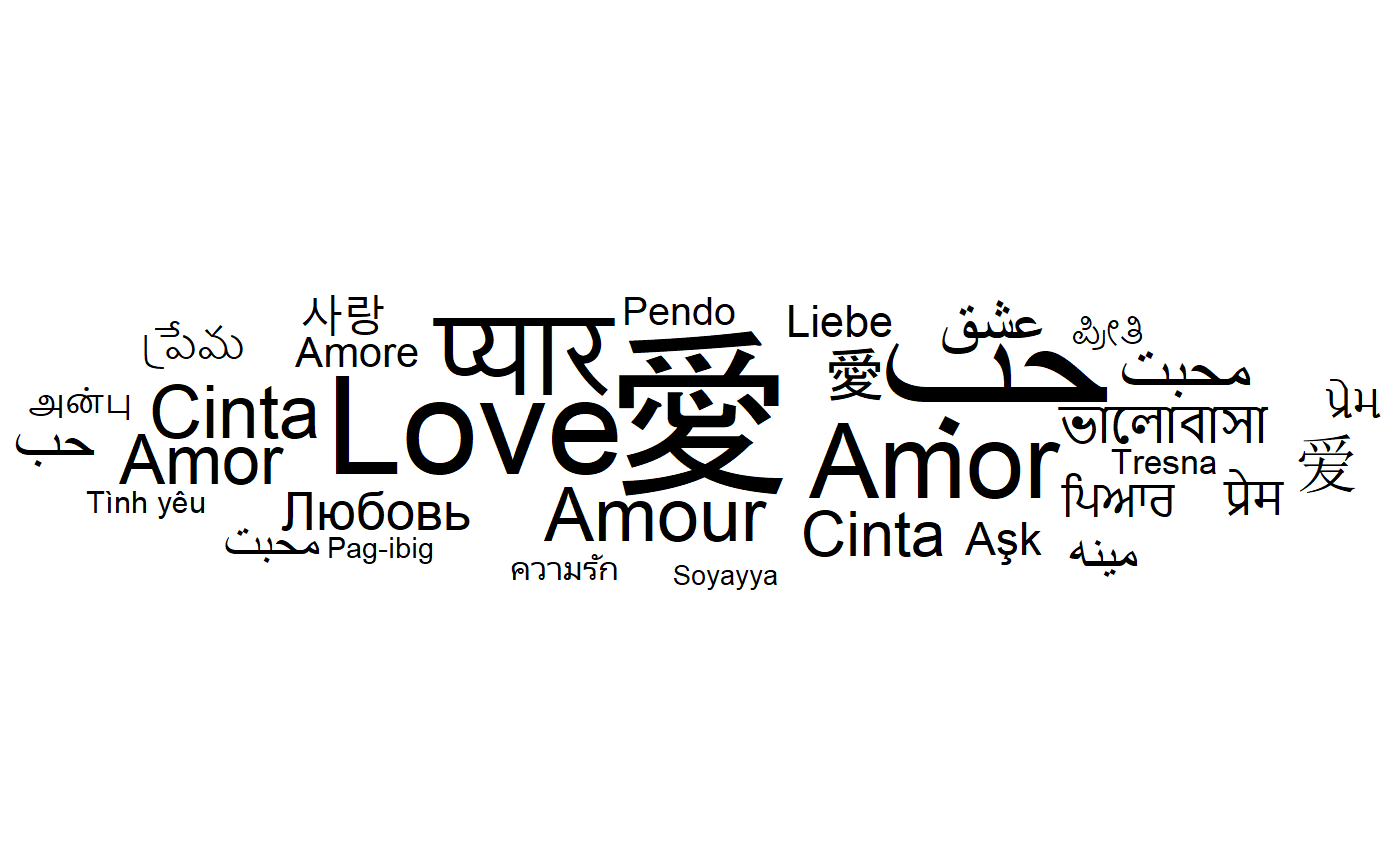

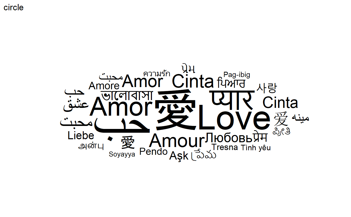
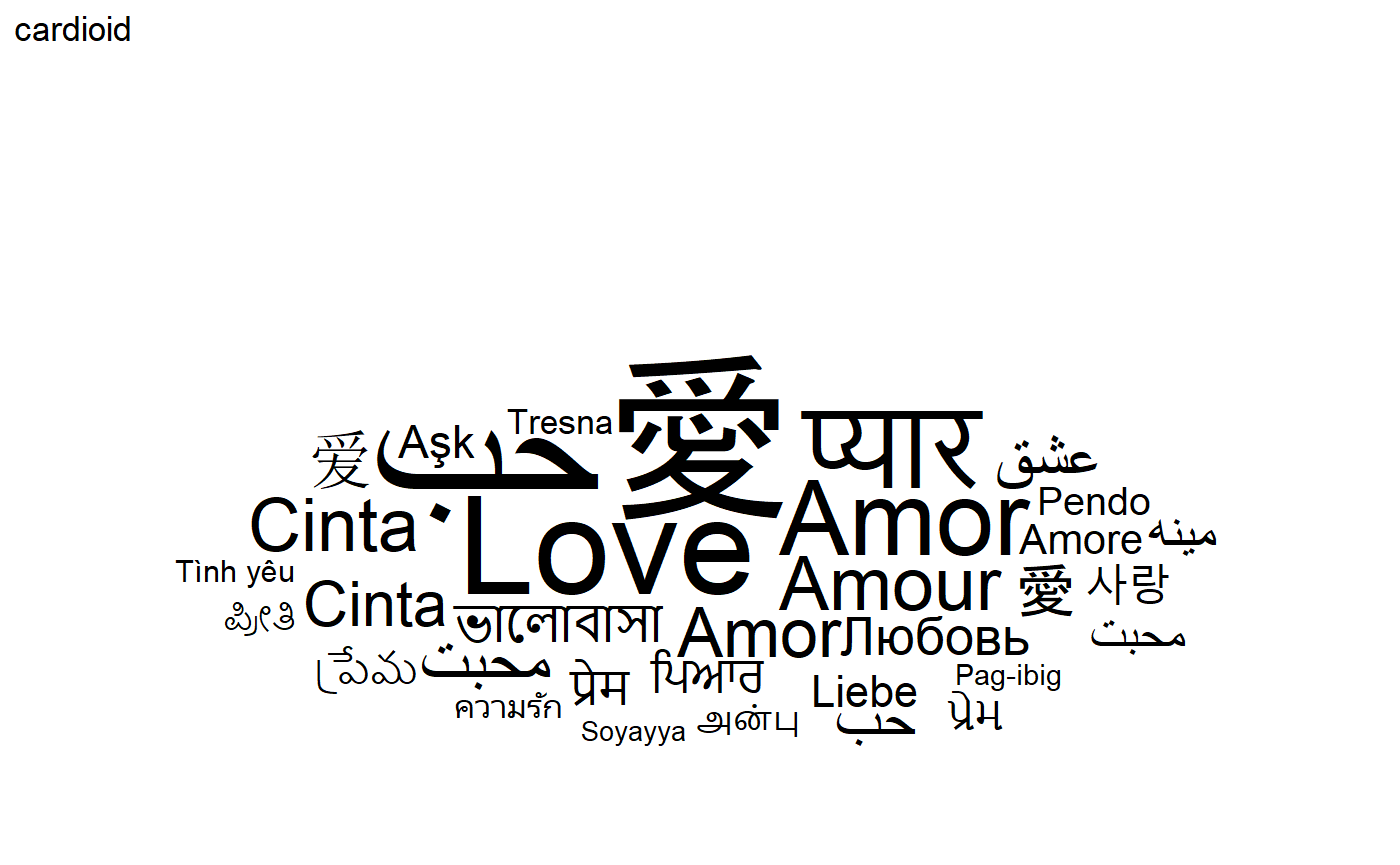
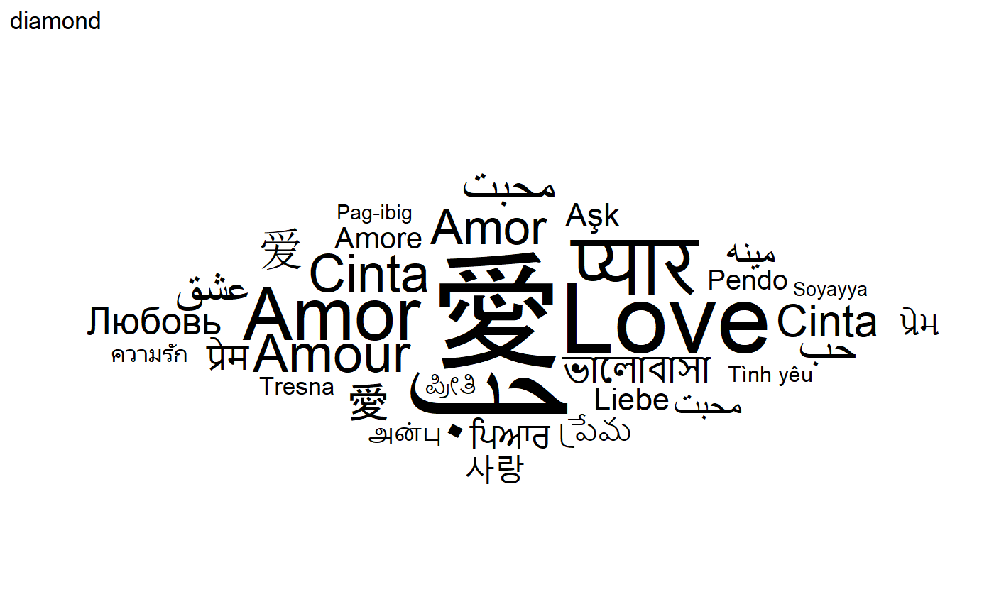
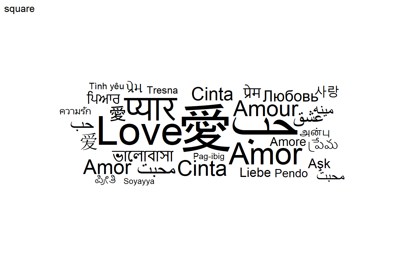
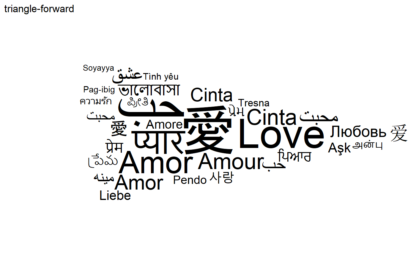
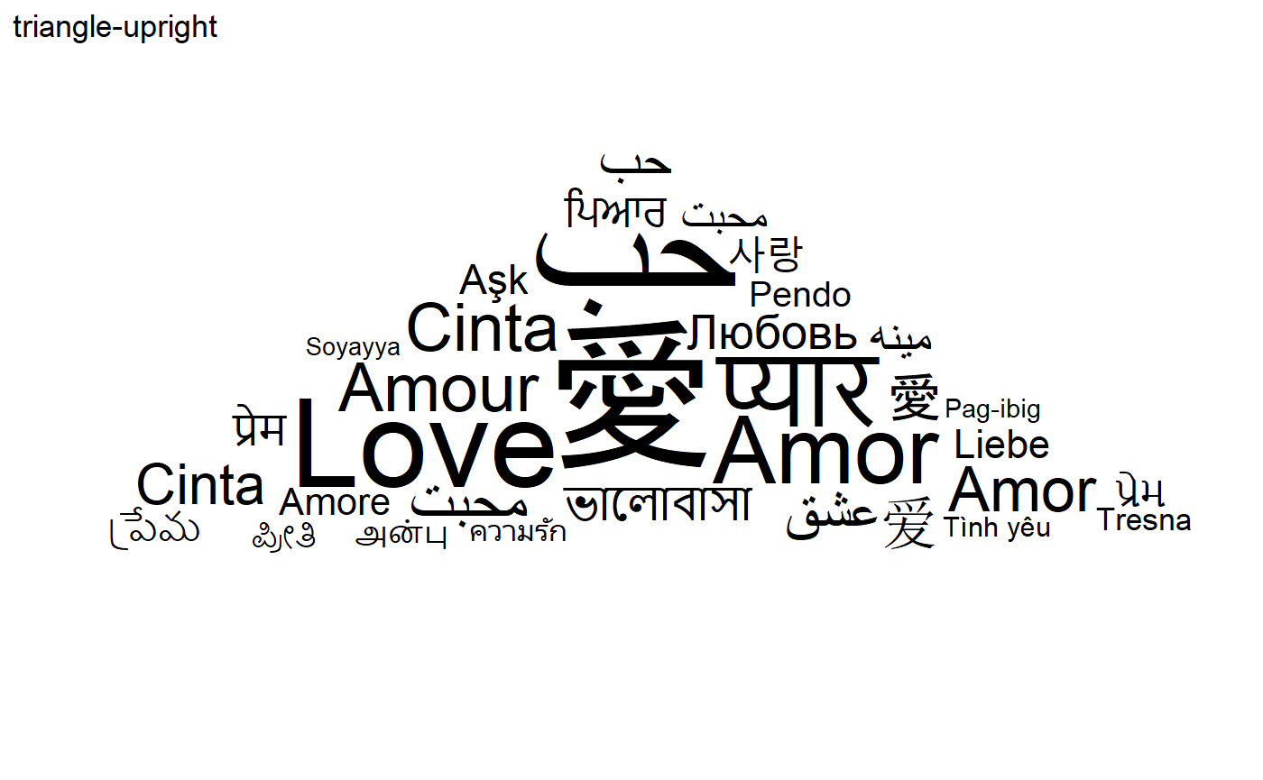
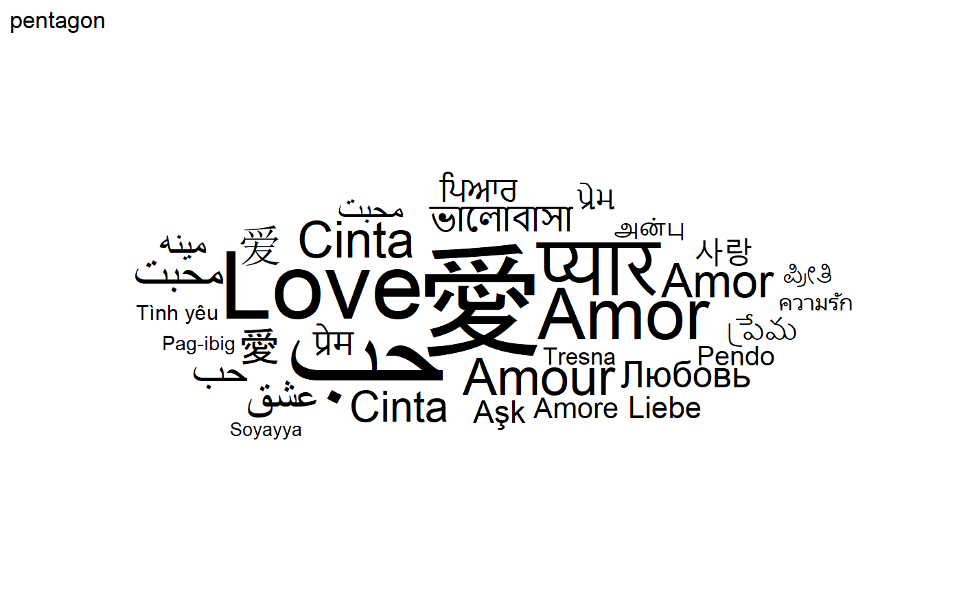
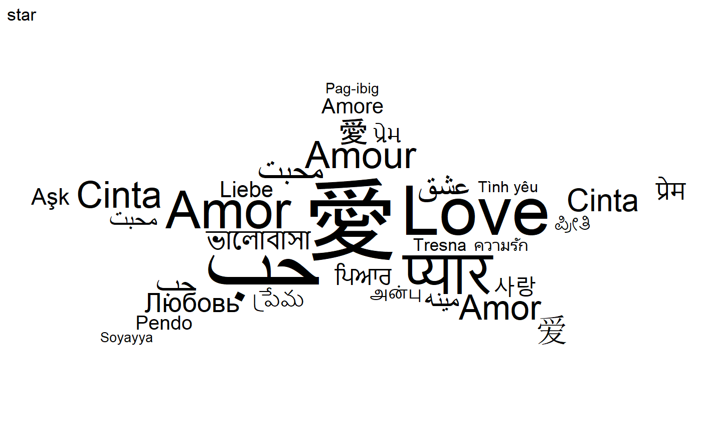
Word cloud and shape

The base shape of ggwordcloud is a circle: the words are place by following a circle spiral. This base shape circle can be change to others (cardioid, diamond, square, triangle-forward, triangle-upright, pentagon or star) using the shape option.

for (shape in c(
  "circle", "cardioid", "diamond",
  "square", "triangle-forward", "triangle-upright",
  "pentagon", "star"
)) {
  set.seed(42)
  print(ggplot(love_words_small, aes(label = word, size = speakers)) +
    geom_text_wordcloud_area(shape = shape) +
    scale_size_area(max_size = 40) +
    theme_minimal() + ggtitle(shape))
}

Word cloud and color

A color can be assign to each word using the color aesthetic. For instance, one can assign a random factor to each word:

set.seed(42)
ggplot(
  love_words_small,
  aes(
    label = word, size = speakers,
    color = factor(sample.int(10, nrow(love_words_small), replace = TRUE)),
    angle = angle
  )
) +
  geom_text_wordcloud_area() +
  scale_size_area(max_size = 40) +
  theme_minimal()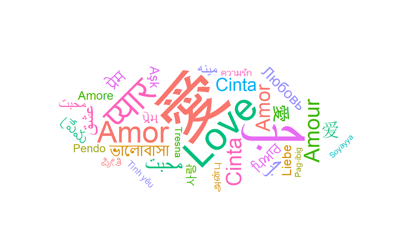

One can also map the color to a value, for instance the number of speakers, and chose the colormap with a scale_color_* scale:

set.seed(42)
ggplot(
  love_words_small,
  aes(
    label = word, size = speakers,
    color = speakers, angle = angle
  )
) +
  geom_text_wordcloud_area() +
  scale_size_area(max_size = 40) +
  theme_minimal() +
  scale_color_gradient(low = "darkred", high = "red")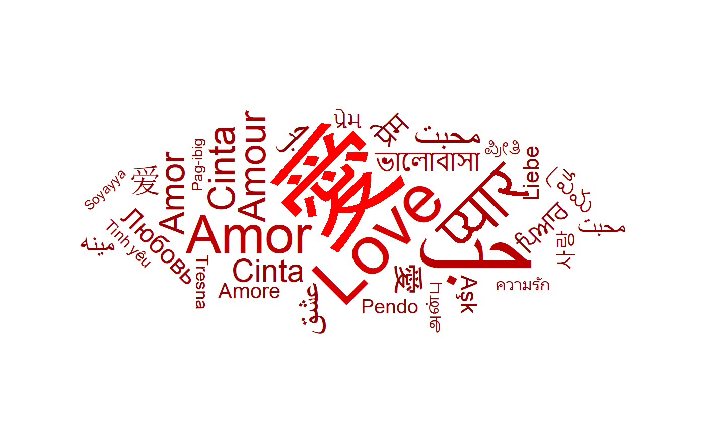

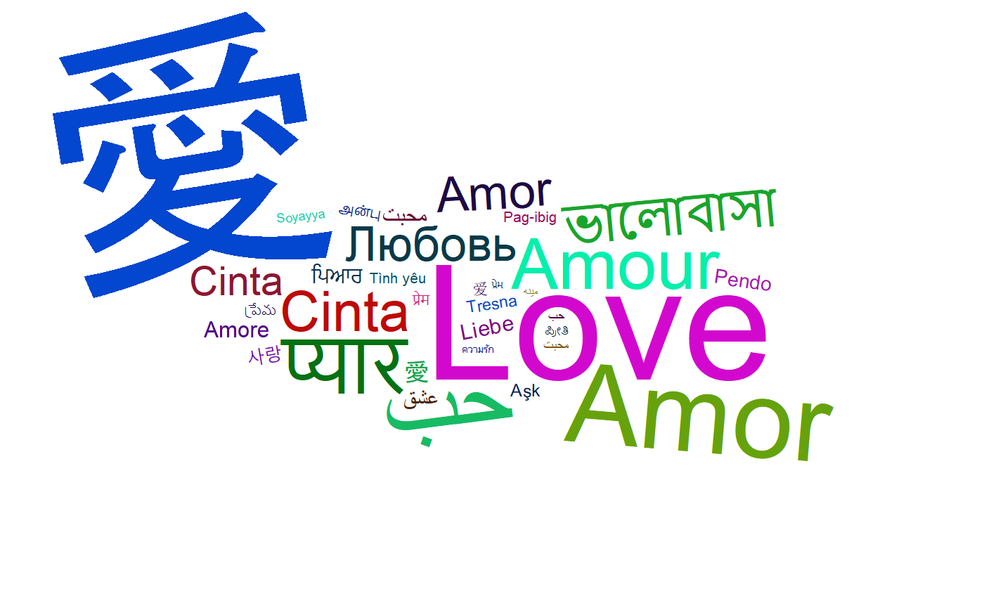
Word cloud and mask

ggwordcloud allows to specify a mask within which the words should be placed. More precisely, the non transparent pixels in an image array (or the black pixel if there is no transparency) will be used as a mask:

set.seed(42)
ggplot(love_words_small, aes(label = word, size = speakers)) +
  geom_text_wordcloud_area(
    mask = png::readPNG(system.file("extdata/hearth.png",
      package = "ggwordcloud", mustWork = TRUE
    )),
    rm_outside = TRUE
  ) +
  scale_size_area(max_size = 42) +
  theme_minimal()
#> Warning in wordcloud_boxes(data_points = points_valid_first, boxes = boxes, :
#> Some words could not fit on page. They have been removed.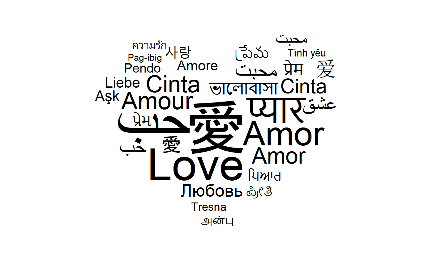

Word cloud with almost everything

We are now ready to make a lovely word cloud:

love_words <- love_words %>%
  mutate(angle = 45 * sample(-2:2, n(), replace = TRUE, prob = c(1, 1, 4, 1, 1)))

set.seed(42)
ggplot(
  love_words,
  aes(
    label = word, size = speakers,
    color = speakers, angle = angle
  )
) +
  geom_text_wordcloud_area(
    mask = png::readPNG(system.file("extdata/hearth.png",
      package = "ggwordcloud", mustWork = TRUE
    )),
    rm_outside = TRUE
  ) +
  scale_size_area(max_size = 40) +
  theme_minimal() +
  scale_color_gradient(low = "darkred", high = "red")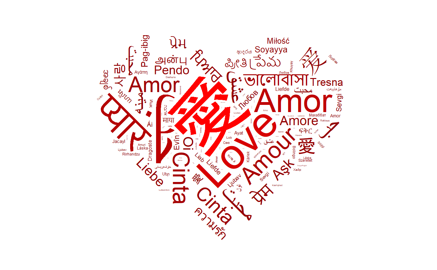

Modified label content and markdown/html syntax

With the label_content aesthetic, cne can specify a different label content than the one used to compute the size. Note that this is equivalent to replace label when not using the text area option.

set.seed(42)
ggplot(love_words_small, aes(label = word, size = speakers,
                             label_content = sprintf("%s (%g)", word, speakers))) +
  geom_text_wordcloud_area() +
  scale_size_area(max_size = 30) +
  theme_minimal()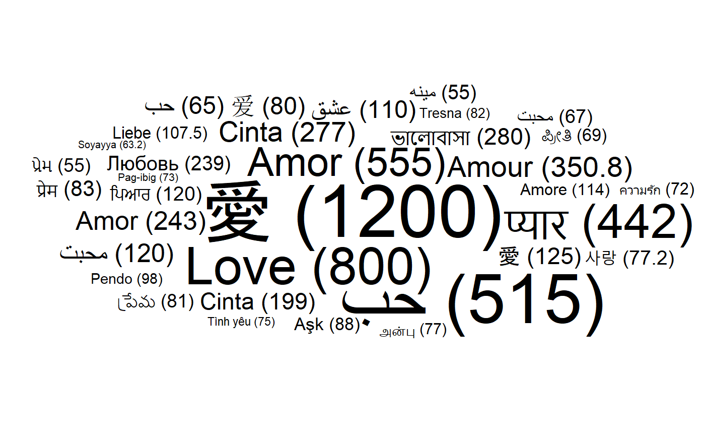

We can combined this with the markdown/html syntax of gridtext to obtain the nicer

set.seed(42)
ggplot(love_words_small, aes(label = word, size = speakers,
                             label_content = sprintf("%s<span style='font-size:7.5pt'>(%g)</span>", word, speakers))) +
  geom_text_wordcloud_area() +
  scale_size_area(max_size = 40) +
  theme_minimal()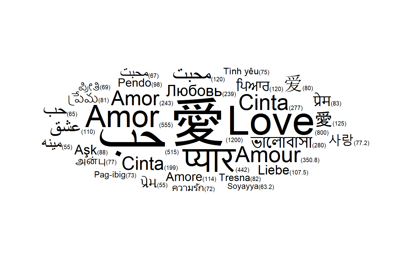

Advanced features

geom_text_wordcloud is compatible with the facet system of ggplot2. For instance, one can easily display two word clouds for the speakers and the native speakers with the same scales:

library(dplyr, quietly = TRUE, warn.conflicts = FALSE)
library(tidyr, quietly = TRUE)
love_words_small_l <- love_words_small %>%
  gather(key = "type", value = "speakers", -name, -word, -angle, -iso_639_3) %>%
  arrange(desc(speakers))

set.seed(42)
ggplot(
  love_words_small_l,
  aes(label = word, size = speakers)
) +
  geom_text_wordcloud_area() +
  scale_size_area(max_size = 30) +
  theme_minimal() +
  facet_wrap(~type)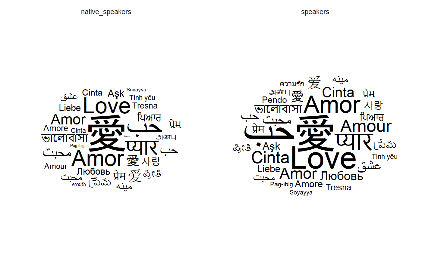

One can also specify an original position for each label that what will be used as the starting point of the spiral algorithm for this label:

set.seed(42)
ggplot(
  love_words_small_l,
  aes(
    label = word, size = speakers,
    x = type, color = type
  )
) +
  geom_text_wordcloud_area() +
  scale_size_area(max_size = 30) +
  scale_x_discrete(breaks = NULL) +
  theme_minimal()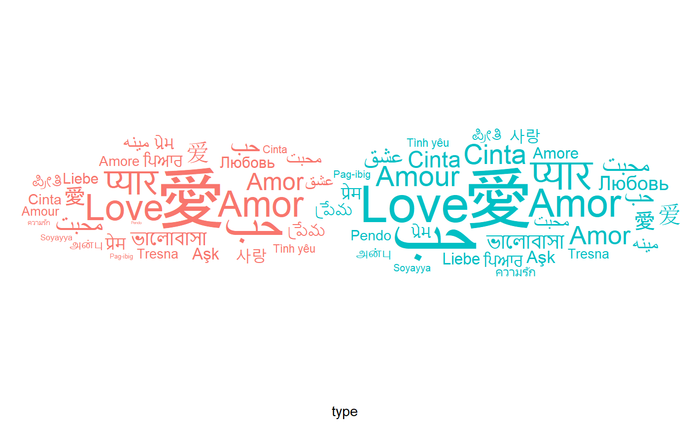

Finally, there is a angle_group option that can be used to restrict the words to appear only in a angular sector depending on their angle_group. For instance, we will visualize the changes of proportions of each language between the speakers and the native speakers by displaying the words above the horizontal line if the proportion is greater than in the other category and below otherwise.

love_words_small_l <- love_words_small_l %>%
  group_by(type) %>%
  mutate(prop = speakers / sum(speakers)) %>%
  group_by(name, word) %>%
  mutate(propdelta = (prop - mean(prop)) / sqrt(mean(prop)))

set.seed(42)
ggplot(
  love_words_small_l,
  aes(
    label = word, size = abs(propdelta),
    color = propdelta < 0, angle_group = propdelta < 0
  )
) +
  geom_text_wordcloud_area() +
  scale_size_area(max_size = 30) +
  theme_minimal() +
  facet_wrap(~type)

ggwordcloud as an approximate replacement for wordcloud and wordcloud2

ggwordcloud and ggwordcloud2 are two approximate replacements for respectively wordcloud and wordcloud2. They provide a similar syntax than the original functions and yields similar word clouds, but not all the options of the original functions are implemented. Note that both use a font size proportional to the raw size aesthetic rather than its square root.

set.seed(42)
ggwordcloud(love_words_small$word, love_words_small$speakers)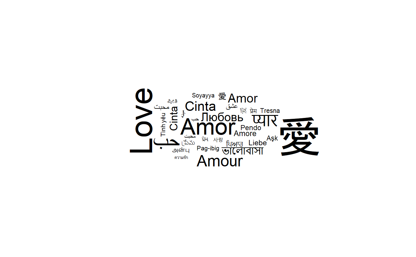

set.seed(42)
ggwordcloud2(love_words_small[, c("word", "speakers")], size = 2.5)