From Parallel Plot to Radar Plot

ggplot2 provides a very elegant way to describe graphics. In this example, we will use its grammar to show how the parallel plot and the radar plot are related.

Our example relies on the mtcars dataset. We first need to rescale all the coordinates between \(0\) and \(1\) and to melt the dataset in order to plot it easily with ggplot.

library(tidyverse)

mtcars_pivot <- mtcars |> 
  as_tibble(rownames = "model") |>
  mutate(across(-model, scales::rescale)) |>
  pivot_longer(cols = -model, names_to = "variable", values_to = "value") |>
  mutate(variable = fct_inorder(variable))

We can now use ggplot and its geom_path geometry to obtain a single parallel plot

library("ggplot2")
ggplot(mtcars_pivot, aes(x = variable, y = value)) +
  geom_path(aes(group = model, color = model), size = 2) +
  theme(strip.text.x = element_text(size = rel(0.8)),
        axis.text.x = element_text(size = rel(0.8)),
        axis.ticks.y = element_blank(),
        axis.text.y = element_blank()) +
  xlab("") + ylab("") +
  guides(color = guide_legend(ncol=2))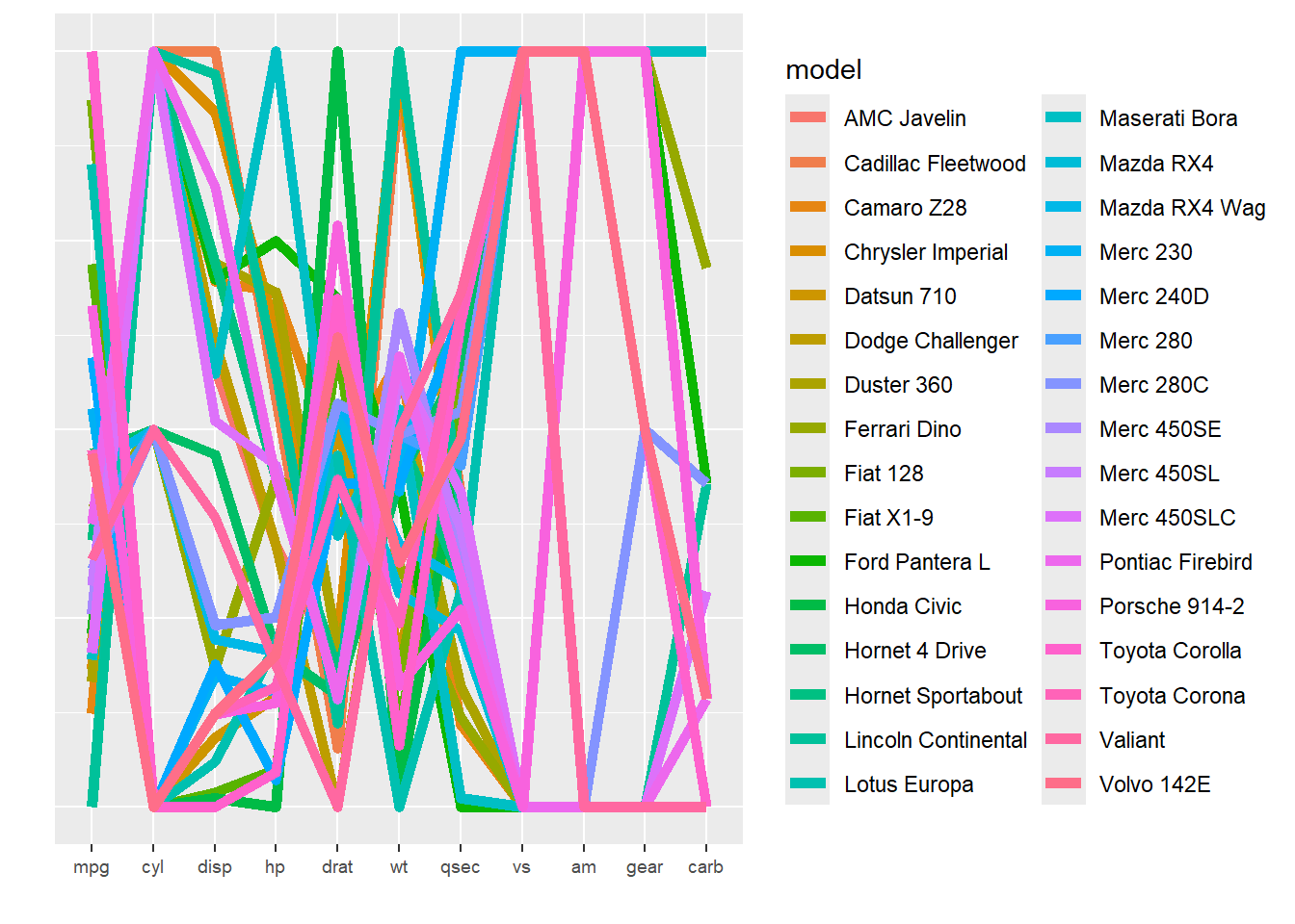

or a small multiple one

ggplot(mtcars_pivot, aes(x = variable, y = value)) +
  geom_path(aes(group = model, color = model), size = 2) +
  facet_wrap(~ model, nrow = 4) +
  theme(axis.ticks.x = element_blank(),
        axis.text.x = element_blank(),
        axis.ticks.y = element_blank(),
        axis.text.y = element_blank()) +
  xlab("") + ylab("") +
  guides(color = "none")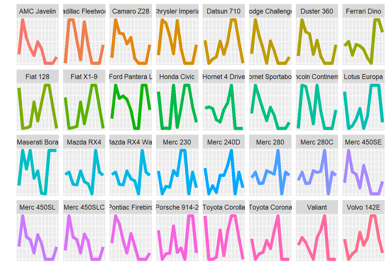

Now the most natural way to convert those figures to a radar plot is to display them in polar coordinates. Indeed, we obtain

ggplot(mtcars_pivot, aes(x = variable, y = value)) +
  geom_path(aes(group = model, color = model),  size = 2) +
  theme(strip.text.x = element_text(size = rel(0.8)),
        axis.text.x = element_text(size = rel(0.8)),
        axis.ticks.y = element_blank(),
        axis.text.y = element_blank()) +
  xlab("") + ylab("") +
  guides(color = guide_legend(ncol=2)) +
  coord_polar()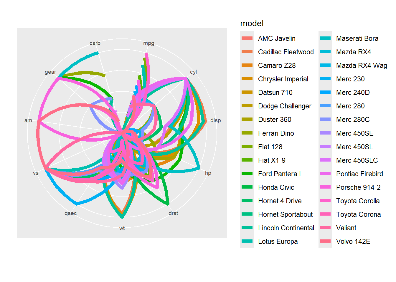

and

ggplot(mtcars_pivot, aes(x = variable, y = value)) +
  geom_path(aes(group = model, color = model), size = 2) +
  facet_wrap(~ model, nrow = 4) +
  theme(axis.ticks.x = element_blank(),
        axis.text.x = element_blank(),
        axis.ticks.y = element_blank(),
        axis.text.y = element_blank()) +
  xlab("") + ylab("") +
  guides(color = "none") +
  coord_polar()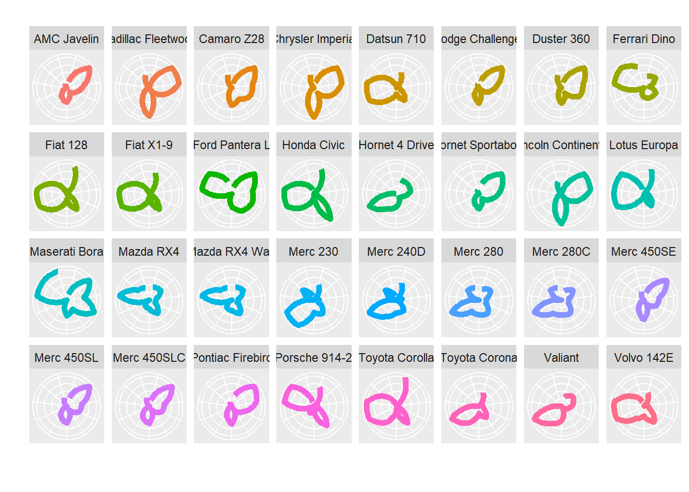

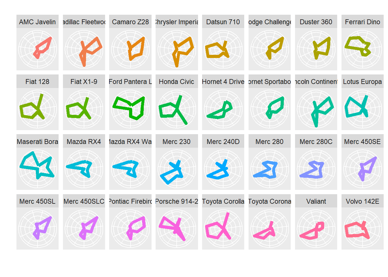
We can see two issues: first the straight lines are converted into curves and second the path is not closed. Those two issues can be solved with ggplot2! For the first one, we will use a trick provided by Hadley Wickham himself and for the second the geom_polygon geometry (as well as geom_path to obtain a nice legend…)

We first define a radar coordinate system:

coord_radar <- function (theta = "x", start = 0, direction = 1) 
{
    theta <- match.arg(theta, c("x", "y"))
    r <- if (theta == "x") 
        "y"
    else "x"
    ggproto("CordRadar", CoordPolar, theta = theta, r = r, start = start, 
        direction = sign(direction),
        is_linear = function(coord) TRUE)
}

ggplot(mtcars_pivot, aes(x = variable, y = value)) +
  geom_polygon(aes(group = model, color = model), fill = NA, size = 2, show.legend = FALSE) +
  geom_line(aes(group = model, color = model), size = 2) +
  theme(strip.text.x = element_text(size = rel(0.8)),
        axis.text.x = element_text(size = rel(0.8)),
        axis.ticks.y = element_blank(),
        axis.text.y = element_blank()) +
  xlab("") + ylab("") +
  guides(color = guide_legend(ncol=2)) +
  coord_radar()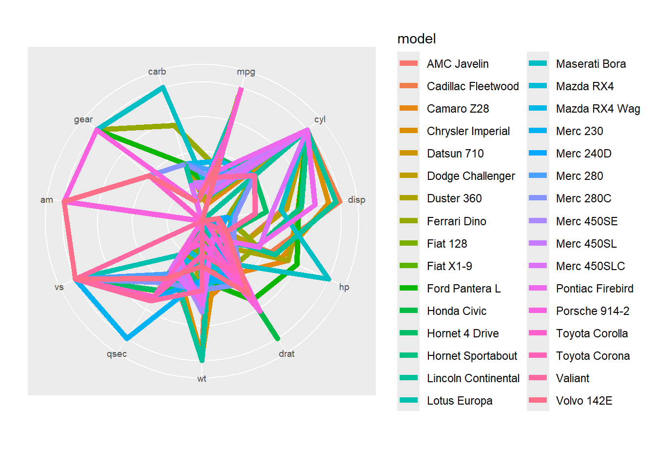

and

ggplot(mtcars_pivot, aes(x = variable, y = value)) +
  geom_polygon(aes(group = model, color = model), fill = NA, size = 2) +
  facet_wrap(~ model, nrow = 4) +
  theme(axis.ticks.x = element_blank(),
        axis.text.x = element_blank(),
        axis.ticks.y = element_blank(),
        axis.text.y = element_blank()) +
  xlab("") + ylab("") +
  guides(color = "none") +
  coord_radar()